Analysis of the dispersion variance using geostatistical simulation and blending piles

 

 

D.M. Marques; J.F. Costa

Federal University of Rio Grande do Sul, Porto Alegre, Brazil

 

 

---

SYNOPSIS

The additive property of dispersion variances was found experimentally by D.G. Krige using data from the gold deposits of the Witwatersrand. In this property, called 'Krige's relationship', the dispersion of a small unit, v, within the deposit is equal to the sum of the dispersion of v within a bigger unit, V, and the dispersion of these units, V, within the deposit, D. It is known that the variance of the grades decreases as the support increases, the so-called volume-variance relationship. To analyse volume-variance and Krige's relationship, the methodology herein proposed combines blending piles and geostatistical simulation to simulate the in situ and the pile grade variability. Variability reduction in large piles is based on the volume-variance relationship, i.e. the larger the support, the smaller the variability (assuming perfect mix). Based on a pre-defined mining sequence to select the blocks that will form each pile for each simulated block model, the statistical fluctuation of the grades derived from real piles can be simulated. Using this methodology, one can evaluate within a certain time period the expected grade variability for various pile sizes, and also calculate the Krige's relationship between the small blocks and the piles of different sizes. A real case study using a large Brazilian iron ore deposit illustrates the methodology and demonstrates the validity of the results.

Keywords: dispersion variance, blending piles, simulation, Krige's relationship.

---

 

 

Introduction

All mineral deposits have variable grades in their composition. Depending on the type of mineralization, there are different scales of variability. Various mining methods can be employed to try to reduce this variability, attempt to reduce the dilution that occurs in mining, and remove the waste from the ore, to maintain the mean grade that feeds the processing plant as constant as possible.

Obviously, an optimal mining method exists for each deposit that yields a product of required average grade for downstream processing at a reasonable cost and a suitable rate of production (Parker, 1979). However, there are some cases where a proper mining method is not sufficient to ensure that the ROM (run of mine) has the characteristics desired for the feeding of the processing plant or the final product.

Common to all mining methods is the notion of the selective mining unit (SMU) - the smallest practical volume that can be classified as ore or waste (Parker, 1979). Considering a SMU of small volume, it is natural that there are some with high grades and others with low grades. These differences in grades among SMUs can be measured by the variance of the SMUs. As the size of the SMU increases, it will tend to include a mixture of high and low grades, reducing the variance. Note that the mean remains constant in all cases.

Krige's relationship or additivity of variances (Krige, 1951, 1981) is a volume-variance relationship, found experimentally by D.G. Krige using data from the gold deposits of the Witwatersrand. In this relationship, the dispersion of a small unit, v, within the deposit is equal to the sum of the dispersion of v within a bigger unit, V, and the dispersion of these units, V, within the deposit, D (Dowd, 1993).

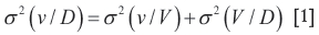
The relationship between these three variances is:

Knowing the principles of Krige's relationship and the volume-variance relationship, it would be possible to analyse the reduction of variability using blending piles of various sizes. Blending (homoge-nization) piles can be used as part of a system of quality control in order to reduce the variability of the material fed to the processing plant.

This is possible only because of the heterogeneity of constitution of the material. Heterogeneity is a primary structural property of all matter, i.e. all particulate solids, dry, wet, suspended in water or in air, are heterogeneous. According to Gy (1998), when the portions forming a material are not strictly identical, the material is considered heterogeneous. The heterogeneity can be analysed from two different aspects, namely relating to the constitution and to the distribution of the material. The heterogeneity of the constitution refers to the intrinsic characteristics of the material, and consists of the differences that exist between particles or constituent fragments of a lot, L. The mixing or blending of the constituent particles of the lot does not have any influence on the heterogeneity of the constitution. This heterogeneity is responsible for the occurrence of the Fundamental Sampling Error.

In order to reproduce the fluctuations in grades (heterogeneity of constitution and distribution) within an orebody (for a daily, monthly, or other time period), conditional simulations can be used (Journel, 1974). By applying this technique, the grades with their spatial continuity and variability are reproduced in models that mimic the real deposit. Some previous investigations involving blending, homogenization piles and geostatistical simulations can be found in Abichequer et al. (2010), Beretta et al. (2010), Binndorf (2013), Costa et al. (2007), Marques et al. (2009), Marques and Costa (2013), and Ribeiro et al. (2008). The seminal work by Schofield (1980) addresses homogenization piles using linear geostatistics (ordinary kriging).

This work presents a study developed on two iron ore deposits located in the Iron Quadrangle region of Brazil. The aim is to investigate the volume-variance relationship for different SMUs (blending piles) with Krige's relationship (analytical solution) and compare it with the results obtained using a numerical simulation. The variable silica (SiO₂ in %) was chosen for this analysis, as it constitutes the most critical contaminant for this iron ore.

 

Methodology

The grades of silica in the feed to the processing plant often fluctuate too much. The first decision is whether to use blending piles (homogenization), and if used, what is the ideal size. To help answer these questions, this study proposes the use of multiple geostatistical simulated models (Journel, 1974) allied to mine planning. Using the sequence of blocks extracted, obtained by mining planning, the fluctuations of the grades in each simulation can be evaluated and a band of uncertainty defined for the grades, considering all possible simulated scenarios.

Multiple outputs provide the means to evaluate the variability of the SiO2 head grades feeding the processing plant. From this temporal sequence emulating the grades feeding the plant it is possible to analyse the volume-variance relationship, as well the dispersion variance of the blocks in the blending piles.

The original data (drill-holes) was used to simulate the grades, simulate the time series, and reconcile the models against the reference values obtained from the historical data from the blocks mined in one year. The simulations in a mining context mimic the characteristics of the mineral deposit, creating an array of values with the same statistical and spatial characteristics as the true grades. A simulation, therefore, is not an estimate, but rather a set of values with the same general statistical characteristics as the original data.

The steps involved in this study are:

> Generation of multiple equally-probable 3D models (geostatistical simulations)

> Sequencing of the simulated 3D block model according to the production of one year

> Emulation of the feeding of the blending (homogenization) piles

> Calculation of the reduction of the variability in blending piles using Krige's relationship (dispersion variance v/V)

> Emulation of the blending piles and calculation of the reduction of variability

> Comparison of the results obtained in the previous two steps.

Assessing block grade uncertainty

A conditional geostatistical simulation algorithm was applied to generate 50 equally probable scenarios of SiO₂ spatial distribution in 10 × 10 × 10 m blocks. Combining the block sequence from the two mines provides the grades which will feed the blending piles, i.e. one block of 1000 m³ from each mine resulting in a 2 000 m³ combined volume (new SMU or v). Grades are shown in a time series (Figure 1) sequentially through a year (as the historical data of the company). Each SMU in this time series has a volume of 2 000 m³ and a mass of approximately 7 173 t. The band of uncertainty associated with each SMU grade (maximum and minimum grades) is obtained through the simulated grades of silica (SiO₂) for each block derived from the 50 equally probable scenarios ordered according to the mine scheduling.

 

 

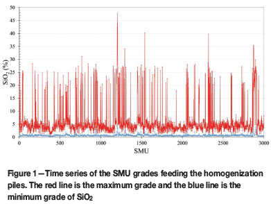
Note the uncertainty in the grades (max-min.) and their fluctuation through the year. These time series values are required as the input to the algorithm used to simulate the homogenization piles allowing an assessment on the reduction of variability.

Inter-pile grade variability using a numerical solution

According to Marques and Costa (2013), each block grade differs from every other, and differs from the global mean of the blocks calculated for the entire year. By grouping various blocks and forming a pile, the average grade of each pile is moved closer to the global annual mean when compared to the grade of each individual block within a pile. This phenomenon explains why the grades in the reclaimed ore from the piles have less variance than the grades that would be obtained from a block-by-block scheme feeding the processing plant.

The first step is to calculate the reduction in the variability. To find the acceptable grade interval we need first to calculate the weighted mean grade using all blocks from the first geostatistical simulation, according to:

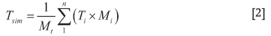
where T_sim is the mean grade of a geostatistical simulation, M_t is the sum of the masses of all blocks in the simulated model, T_i is the grade of the block I, M_i is the mass of the ith block, and n is the number of existing blocks in the geostatistical simulation.

Next, we need to calculate the weighted mean grade of each pile (for the same simulation) according to:

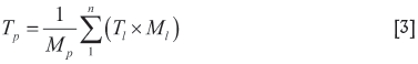
where T_p is the mean grade of the pile, M_p is the total mass of the pile, T_l is the grade of the block I, M_l is the mass of the block l, and n is the number of blocks forming the pile.

For each pile formed, the squared difference between the pile mean grade and the mean grade of the simulation (T_sim) (all blocks throughout the year) is calculated. Next, these squared differences are averaged, leading to the variance of the pile grades throughout the year, for the mass of the homogenization pile selected (inter-pile variance). The entire process then starts again, but choosing a different simulation.

Inter-pile grade variability using Krige's relationship

In many practical situations, it is necessary to know a regionalized variable which is the average over a certain volume or area, rather than at a point. The basic volume on which a regionalized variable is measured is called its support (Armstrong, 1998). When a change occurs in the support (increase), a new block size is created. This new block or SMU is related to the previous one via the global average, but their spatial structural characteristics are different. For example, simulations in blocks of 10 × 10 × 10 m have greater variability than the panel (combination of blocks) created by blending these blocks. As the support increases, the variability among the new panels (combination of various blocks) decreases. The question we need to answer is how much this variability changes at different supports.

Using Krige's relationship, the dispersion variance of the SMUs (v) within each panel (V) was measured. Knowing the total variance for the year (v/D), it is possible to compute the variance among piles over the year (v/D).

In this analysis, let us consider v, the smallest panel, as 2 000 m³, or approximately 7 173 t, which is the size of the SMU; the unit V as the different panels tested (from approximately 7 173 t to 1 000 kt - equivalent to the various pile sizes tested); and D as the whole domain (comprising the sum of the 3 000 panels of 2 000 m³ each). For calculation purposes, the panel is considered as a function of the volume of individual SMUs (same volume support, i.e. constant in each block), but all results are presented as a function of the mass (approximate). Block mass may vary depending on the density of the rock type predominant at each SMU.

The reduction in variability due to the increase in the mass can be calculated from the dispersion variance, according to:

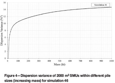
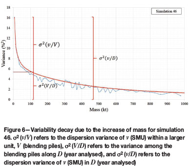
where s²(v/V) is the dispersion variance of v (SMU) within a bigger unit V (blending pile), (v/v) is the variance of v (SMU) through the year, and (V/V) is the variance of a bigger unit V (blending piles) in the year.

Initially (v/v) and (V/V) are calculated. This can be done using the appropriated charts (Journel and Huijbregts, 1978) or obtained by averaging the variogram value between all possible pairs within a SMU (known as a 'gammabar'; Deutsch and Journel, 1998). For other examples on calculating dispersion variance, see Isaaks and Srivastava (1989), Pyrcz and Deutsch (2002), and Journel and Kyriakidis (2004). In this case, the value of s²(v/D) is known for each simulation analysed, and is equal to the variance of the time series (grades of the continuous flow feeding the processing plant).

Thus, for each simulation of a continuous flow of ore that feeds the processing plant, or a blending and/or homogenization stack, it is necessary to calculate the experimental variogram of the grades and model it. As each simulation of continuous flow is a possible representation of reality, and all are slightly different, there are 50 possible temporal variograms. In the following discussion the variograms for just two of them are presented (simulations #30 and #46), which can be seen in Figure 2a and Figure 2b. In these figures, the variogram model is represented by a continuous black line. The lag used in the calculation of the experimental variogram (or chrono-variogram) for the continuous flow grades is approximately 2 hours and 55 minutes.

 

 

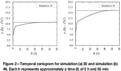
The variogram model can be seen in Equations [4] and [5] for simulations no. 30 and no. 46, respectively.

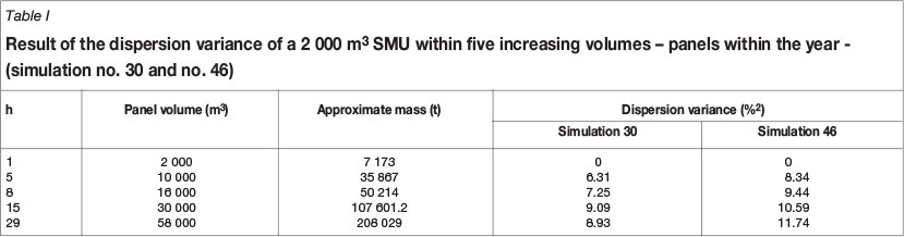
where each model is represented by a nugget effect, Co, two spherical structures (Sph) with C1 and C2 as their sill contribution, and ranges, a1 and a21, respectively [g(h) = Co + C1*Sph (h/a1) + C2*Sph(h/a2)]. Once the variogram for each simulation has been fitted, it can be further used to calculate the dispersion variance. Table I presents the results for five panels (combination of multiple blocks sizes) using simulations no. 30 and no. 46.

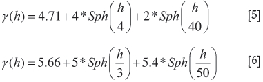
Figure 3 and Figure 4 show the complete results for the dispersion variance of 2 000 m³ SMUs within increasing pile sizes (or equivalent panel volumes) for simulations no. 30 and no. 46, respectively.

 

 

 

 

Results

The variance of the final grade which feeds the processing plant is the sum of variability of the sources s²(v/V) and s²(V/D). Figure 4 depicts the values for the total variability (s²) of the grades due to the two sources listed versus the different blending pile sizes. The variability reduction associated with the increase of mass using the dispersion variance formula (area above the line) is shown in red (continuous smooth line). The blue (jagged) line is the variability decay due to the increase of mass for different pile sizes using the numerical solution (numerical emulation of the pile grades). Note that although the blue line is less smooth than the red line, both share the same overall form. Also, Figure 5 and Figure 6 have different total variances (y-axis), but are equivalent in form and proportion.

 

 

 

 

The benefit of reducing the variability of the head grades obtained by using different blending pile sizes can be seen clearly in Figure 4. For instance, a 50 kt pile will lead to a reclaimed ore with a head grade variance approximately 50% less than would be obtained by feeding the plant directly with the grades of 7 173 t SMUs.

The calculation on variability reduction due to the increase in pile mass was repeated for 50 equally probable simulated block models using either Krige's relationship or numerical emulation (Marques and Costa, 2013). For the sake of comparison the resulting total variance of each simulation was standardized (equal to 1). Figure 7 shows the results using Krige's relationship, and Figure 8 shows the results for the numerical simulation.

 

 

 

 

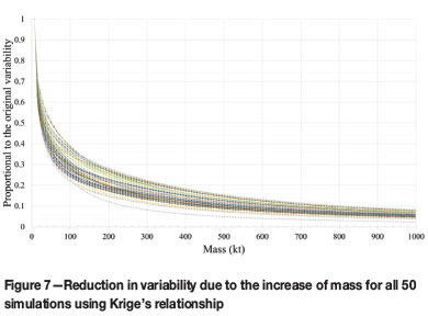
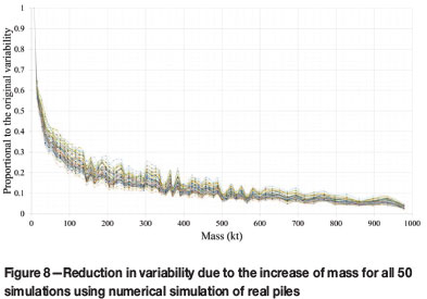
The plots suggest an exponential decay in grade variability with an increase in pile size. This reproduces the volume-variance relationship discussed in Parker (1979). Consequently, the grades measured in the reclaimed ore from the piles will have a reduced variance when compared to the grade variability that would be obtained from feeding the processing plant block-by-block (or SMU-by-SMU).

It should be kept in mind that this reduction in variability will be obtained only if properly designed and operated homogenization piles (of the proper size and with the proper number of layers) are in place. This analysis is based on the heterogeneity of distribution, i.e. the way the material is distributed within a pile. The parts forming the stack differ among themselves and are different from the average content of the stack. Organizing the block or SMU forming the stack in different numbers of layers leads to a reduction of variation in the grades that will feed the processing plant. For each increment of mass, it is possible obtained a new time series of the feed to the processing plant (from the formed homogenization piles). The larger the homogenization pile that is formed, the lower the uncertainty in this band of the time series (as long as the pile is adequately homogenized). A detailed proof of this topic can be seen in Marques and Costa (2013).

 

Conclusions

The data used for modelling the variogram needed to calculate the variance of dispersion derives from simulated continuous flow and does not have the spatial structure of the original mineral deposit. The grades along the continuous flow follow the mining sequence and no longer have the spatial characteristics of the deposit. However, the sequence of values has its own temporal autocorrelation structure.

The dispersion variance decreases as the support increases. This relationship (volume-variance) is well known and the results corroborate the principle embedded in Krige's relationship. The simulation of a continuous flow was used to model the temporal variogram and to obtain the dispersion variance for various pile sizes. Additionally, a numerical simulation of various pile sizes gave very similar results.

The algorithm designed to predict the variability in the blending piles reflects the uncertainty associated with in situ grades. The use of estimated models (via any Kriging method, for instance) is not suitable for performing this type of analysis, as there is an excessive smoothing in the block grades.

The largest amount of variability reduction in the homogenization system is associated with the mass pile increase (inter-pile grade variability). However, the number of layers should also be also considered in the formation of a homogenization pile, as a pile with a large mass but improperly assembled will not lead to the expected reduction in variability.

 

References

Abichequer, L.A., Costa, J.F.C.L., Pasti, H.A., and Koppe, J.C. 2010. Design of blending piles by geostatistically simulated models - A real case reconciliation. International Journal of Mineral Processing, vol. 99. pp. 21-26.         [ Links ]

Armstrong, M. 1998. Basic Linear Geostatistics. Springer, Berlin.         [ Links ]

Beretta, F.S., Costa, J.F.C.L., and Koppe, J.C. 2010. Reducing coal quality attributes variability using properly designed blending piles helped by geostatistical simulation. International Journal of Coal Geology, vol. 84, no. 2. pp. 83-93.         [ Links ]

Binndorf, J. 2013. Application of efficient methods of conditional simulation for optimising coal blending strategies in large open pit mining operations. International Journal of Coal Geology, vol. 112. pp. 141-153.         [ Links ]

Costa, J.F.L.C., Koppe, J.C., Marques, D.M., Costa, M.S.A., Batiston, E.L., Pilger, G.G., and Ribeiro, D.T. 2007. Incorporating in situ grade variability into blending piles design using geoestatistical simulation. Proceedings of the Third World Conference on Sampling and Blending, Porto Alegre, Brazil, 23-25 October 2007. Costa, J.F.C.L. and Koppe, J.C. (eds.), Fundacao Luiz Englert. pp. 378-389.         [ Links ]

Deutsch, C.V. and Journel, A.G. 1998. GSLIB. Geostatistical Software Library and User's Guide. 2nd edn. Oxford University Press.         [ Links ]

Dowd, P.A.1993. Basic Geostatistics for the Mining Industry. University of Leeds. (Monograph).         [ Links ]

Gy, P. 1998. Sampling for Analytical Purposes. John Wiley& Sons, Chichester.         [ Links ]

Isaaks, E.H. and Srivastava, M.R. 1989. An Introduction to Applied Geostatistics. Oxford University Press, New York.         [ Links ]

Journel, A.G. 1974. Geostatistics for conditional simulation of ore bodies. Economic Geology, vol. 69, no. 5. pp. 673-687.         [ Links ]

Journel, A.G. and Huijbregts, C.J. 1978. Mining Geostatistics. Academic Press, New York.         [ Links ]

Journel, A.G. and Kyriakidis, P.C. 2004. Evaluation of Mineral Resources: A Simulation Approach. Oxford University Press, New York.         [ Links ]

Krige, D.G. 1951. A statistical approach to some mine valuation and allied problems on the Witwatersrand. MSc thesis, University of the Witwatersrand, Johannesburg.         [ Links ]

Krige, D.G. 1981. Lognormal-de Wijsian Geostatistics for Ore Evaluation. South African Institute of Mining and Metallurgy, Johannesburg.         [ Links ]

Marques, D.M., Costa, J.F.C.L., Ribeiro, D.T., and Koppe, J.C. 2009. The evidence of volume variance relationship in blending and homogenisation piles using stochastic simulation. Proceedings of the Fourth World Conference on Sampling and Blending. Cape Town, South Africa, 21-23 October 2009. Southern African Institute of Mining and Metallurgy, Johannesburg. pp. 235-242.         [ Links ]

Marques, d.M. and Costa, J.F.C.L. 2013. An algorithm to simulate ore grade variability in blending and homogenization piles. International Journal of Mineral Processing, vol. 120. pp. 48-55.         [ Links ]

Parker, H. 1979. The volume variance relationship: a useful tool for mine planning. Engineering and Mining Journal, vol. 180. pp. 106-123.         [ Links ]

Pyrcz, M.J. and Deutsch, C.V. 2002. Geostatistical Reservoir Modeling. Oxford University Press, New York.         [ Links ]

Ribeiro, D.T., Roger, L.S., Vidigal, M., Costa, J.F.C.L., and Marques, d.M. 2008. Conditional simulations to predict ore variability and homogenization pile optimal size: a case study of an iron deposit. Proceedings of the Eighth International Geostatistics Congress, Santiago, Chile, 1-5 December 2008. Ortiz J.M. and Emery X. (eds.). pp. 749-758.         [ Links ]

Schofield, e.G. 1980. Homogenisation/Blending Systems Design and Control for Minerals Processing. TransTech Publications, Zurich.         [ Links ]