


Servicios Personalizados
Articulo
 Inglés (pdf)
 Articulo en XML
 Referencias del artículo
Indicadores

Links relacionados
-
 Citado por Google
 -
 Similares en Google
Compartir

 Permalink
Journal of the Southern African Institute of Mining and Metallurgy
versión On-line ISSN 2411-9717
versión impresa ISSN 2225-6253
J. S. Afr. Inst. Min. Metall. vol.114 no.6 Johannesburg jun. 2014
GENERAL PAPERS
A methodology for determining the erosion profile of the freeze lining in submerged arc furnace
H. Dong; H.-J. Wang; and S.-J. Chu
School of Metallurgical and Ecological Engineering, University of Science and Technology Beijing, Beijing, China
SYNOPSIS
This paper presents a heat conduction model to determine the erosion profile of freeze linings in a ferronickel submerged arc furnace. Kirchhoff transformation was adopted to simplify the nonlinear equation governing heat conduction. The boundary element method (BEM) and Nelder-Mead simplex optimization method were employed to solve an inverse heat conduction problem. Erosion profiles could be obtained when calculated temperatures at sensor locations agreed well with measured temperatures. The model was validated by comparing the heat loss through the linings, which was calculated by BEM and integral operation after erosion profiles were obtained, with the value calculated from industrial data such as actual power consumption, tap-to-tap time, and ferronickel output. The optimal solution for the erosion profile could be acquired when the difference in heat losses calculated by these two methods is at a minimum.
Keywords: submerged arc furnace, freeze lining, erosion profile, boundary element method.
Introduction
The submerged arc furnace (SAF) is still the predominant route for ferroalloy production, accounting for over 70% of production. SAF campaigns are strongly influenced by the lifetime of the lining, which is gradually eroded or worn due to physical and chemical wear by molten alloy and slag. The design of a SAF is a lengthy process, and construction is expensive. In order to prevent breakouts, it is important to monitor the residual thickness of linings.
To estimate the erosion profile of SAF linings, a few online monitoring models (Kievit et al., 2004; Rodd, Voermann, and Stober, 2010; Karstein and Skaar, 1999) have been developed since 1999, which are similar to that applied in monitoring the erosion of the hearth and bottom of a blast furnace (BF). The methodologies by which information on a BF hearth state is obtained include core sampling (Akihiko, 2003), non-destructive testing (NDT) (Afshin and Pawel, 2009), and theoretical prediction (Zhao et al., 2007; Swartling et al., 2010; Surendra, 2005; Brännbacka and Saxén, 2008; Zagaria, Dimastromatteo, and Colla, 2010; Torrkulla and Saxén, 2000; Lijun and Huier, 2003; Yu and Robit, 2008; Kuncan, Zhi, and Xunliang, 2009; Kouji, Takanobu, and Kouzo, 2001). Thicknesses of linings, provided by core sampling and NDT methods are precise, but these methods have obvious drawbacks. Core sampling requires a furnace shutdown, with consequent loss of production. The thickness of lining acquired by NDT has a local character and cannot represent the status of the entire BF hearth. Theoretical prediction, on the other hand, calculates the location of 1150°C isotherm based on measured temperatures from thermocouples embedded in hearth linings. This isotherm was considered as the wear-line in the BF hearth model. Theoretical prediction models involve a heat conduction model and a composite model that combines heat conduction theory with CFD (Kuncan, Zhi, and Xunliang, 2009). With respect to the heat conduction model, there are two ways to approach a heat transfer problem: direct and inverse heat conduction problems, known as DHCP and IHCP (Swartling et al, 2010). Boundary conditions and thermo-physical properties are known in the DHCP models (Swartling et al, 2010; Surendra, 2005; Lijun and Huier, 2003). A significant limitation of DHCP models is that the computational domain is not immutable. Hence it is necessary to continually change the computing domain, which varies with the location of the erosion boundary. However, it is difficult to accomplish this by the DHCP approach. For instance, Lijun and Huier (2003) attempted to employ BEM to solve a DHCP and the 1150°C isotherm was investigated by the orthogonal design. Either thermo-physical properties or boundary conditions could be known in the IHCP model; instead, interior temperatures had to be known for some points of the domain (Swartling et al, 2010). Monitoring models to solve IHCP and estimate the shape of erosion profile were developed, the system geometry of which is not fully known but is being investigated in the solution. Some investigators (Bránnbacka and Saxén, 2008; Zagaria, Dimastromatteo, and Colla, 2010; Torrkulla and Saxén, 2000) combined the optimization technique with a numerical method to solve IHCP, obtaining several acceptable solutions for the erosion profile. It is important to note that the approximate solutions acquired from IHCP models are not unique. Therefore, validation is very important in numerical simulation because the availability of a computing model should be carefully considered. The most common validating method is the comparison between calculated temperatures and measured temperatures. If calculated temperatures at thermocouple locations approximate measured ones, the solution for the erosion profile can be accepted. Due to the non-uniqueness of solutions in IHCP, some other measurements were employed to validate the computation models in addition to comparison of temperatures. Dig-out investigations (Zagaria, Dimastromatteo, and Colla, 2010; Kouji, Takanobu, and Kouzo, 2001) are also a good validation method, but this process is available only during the blow-out of a BF. Torrkulla and Saxén (2000) validated the model by analysing various hearth phenomena such as pressure drop, coke voidage, production rate, and slag delay. In addition, Yu and Robit (2008) combined the CFD model with a one-dimensional heat conduction to perform a numerical analysis on the inner profile of a BF hearth. However, this calculation procedure is overly complex.
Many researchers have contributed to modelling the complex process of lining erosion in a BF hearth, while only few have paid attention to the erosion profile of SAFs, and monitoring of SAF linings is still in its infancy. Kievit et al. (2004) utilized a one-dimensional steady heat conduction method to monitor a ferromanganese SAF. Rodd, Voermann, and Stober (2010) developed a two-dimensional DHCP model that was used for a SAF for ferronickel production. Karstein and Skaar (1999) exploited two different numerical algorithms and employed the finite element method (FEM) to solve IHCP for an ilmenite melting furnace. The simulated results obtained from this work were validated by the method of temperature comparison.
In view of the lack of methods for determining the erosion profile of the freeze lining in SAFs and the shortcomings of the method of temperature comparison, we have developed a model for monitoring the erosion profile in a ferronickel SAF at the Liang-Da cooperation in Shandong Province, China. Measured temperatures from the thermocouples were utilized to solve an inverse heat conduction problem. The nonlinear differential equation could be converted into a Laplace equation after introducing Kirchhoff transformation. BEM and the Nelder-Mead simplex optimization method (Nelder and Mead. 1965) were adopted simultaneously in order to improve the speed of solution. Furthermore, the computing model was validated with industrial data such as actual power consumption, tap-to-tap time, and output of ferronickel.
Compared with previous monitoring models for SAFs, there are two main advantages in the methodology presented in this paper. Improved accuracy and efficiency are obtained by employing BEM and the Nelder-Mead simplex algorithm, and a new validation method is presented, in which the model is validated utilizing industrial data.
Mathematical model
Governing equations and boundary conditions
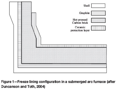
The SAF lining model studied in this paper is built with reference to the configuration illustrated in Figure 1. According to this concept, the ceramic protection layer is a sacrificial layer, and a 'skull' will be formed at the interface between carbon brick and molten iron after the ceramic layer has been eroded away. The erosion profile of the freeze lining could therefore be determined if the inner contour of the carbon brick region could be calculated. Figure 2 illustrates a calculation domain Q to represent the carbon brick region, the inner boundary of which is expressed as B5, and the determination of its shape is the aim of the present work.
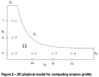
Sensor locations in the system geometry Q are indicated by the open circles in Figure 2. Six thermocouples numbered from 1-6 are utilized to measure internal temperatures. A further six thermocouples, numbered 7-12, are embedded at the interface between carbon brick and graphite to measure the boundary temperature. It should be pointed out that the actual number of sensors in a SAF is larger. In region Q, heat conduction in the steady state can be described by the 2D rotational symmetry equation:
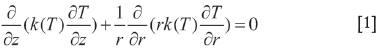
where T is the temperature at a point (r, z), r and z are the radial and axial coordinates, respectively, and k (T ) is the thermal conductivity of the carbon brick, which is a function of temperature as shown in Equation [2] and can be detected by micro-laser flash apparatus (LFA427, NETZSH group, Germany) .

Equation [1] is a nonlinear partial differential equation because the function of thermal conductivity is a logarithmic equation. Kirchhoff transformation (Carslaw and Jaeger, 1959) is applied to simplify the differential equation of heat conduction. A new temperature variation U is used to replace T (Equation [3]), where k0 is thermal conductivity of carbon brick at a known temperature T0. The Laplace equation can be obtained after substituting U into Equation [1] as follows.
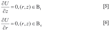
In order to solve Equation [4], boundary conditions should be specified and transferred by Kirchhoff transformation for the domain Q border. Heat fluxes of B1 and B4 are assumed to be zero since the model is rotational symmetric.
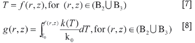
Temperatures of the boundary between B2 and B3 were measured by thermocouples 7-9 and 10-12 respectively. A function f(r, z) was selected to describe the Dirichlet boundary condition of B2 and B3. A new function g(r, z) of boundary conditions could also be established from the Kirchhoff transformation.
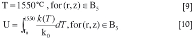
The 1150°C isotherm is defined as the inner boundary when the erosion profile of the BF hearth is monitored. This temperature corresponds to the solidification of the eutectic Fe-C, and the hot metal is in solid state at lower temperatures than this (Kuncan, Zhi, and Xunliang, 2009). In industrial ferronickel production, the FeNi liquidus temperature is around 1300°C and the slag liquidus temperature is 1550°C. Since the amount of slag is very large in ferronickel production, the slag liquidus temperature 1550°C is defined as the hot face boundary condition (Rodd, Voermann, and Stober, 2010.
Numerical and optimization method for inverse heat conduction problem
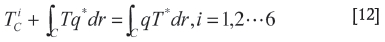
Normally, the solution for IHCP consisted of two main parts. First, a numerical method was utilized to calculate the temperatures at the sensor locations, and an optimization method was then adopted to minimize the difference between the calculated temperature (TC) and measured temperature (TM) (Equation [11]). The unknown erosion profile will be estimated by this computation scheme, illustrated as Equation [11]:
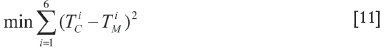
where Tc is the temperature calculated by the numerical methods, TM is the measured temperature from the thermocouples, and superscript i is the number of thermocouples in domain Ω.
The Laplace equation describing the domain Ω. in Figure 2 could be solved by BEM with high efficiency. Temperatures at the thermocouple locations could be calculated from Equation [12]. The integrating range C consists of the entire boundary (B1∪B2∪B3∪B4∪B4∪). T* represents the fundamental solution of the Laplace equation and q* is its derivative (Kurpisz and Nowak, 1995).
The inside boundary B5, as the optimizing object, should be determined by some parameters at first. The parameterization schedule to B5 is shown in Figure 3 and described as follows.
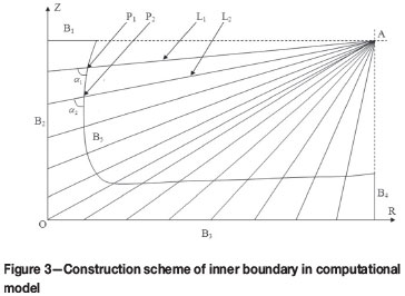
Two straight lines were extended from the B1 and B4 boundary, which intersect at structure point A. Structure lines (L1, L2, L3, ... Ln) were built after connecting point A with some points on B2 and B3. B5 would be formed by cubic spline interpolation to boundary points (P1, P2, P3, ... Pn) that lie on the structure lines. Because the relationship between r and z is linear on the structure lines, a set of radial coordinates (r1, r2, r3, ... rn) of boundary points is defined as optimizing parameters. The ill-posed property is a major obstacle in the solution process. Small changes in measured data would lead to significant fluctuations. In order to prevent the emergence of unreliable solutions, a regular-ization method was adopted to modify the equation (Brännbacka and Saxén, 2008; Zagaria, Dimastromatteo, and Colla, 2010; Torrkulla and Saxén, 2000). Therefore, instead of the minimizing formula in Equation [11], the minimization process was modified with a regularizer, as shown in Equation [13].
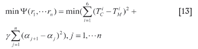
where Ψ is the objective function, j is the number of boundary points, aj is the angle between structure line and B5, and γ is a regularization term. The Nelder-Mead simplex optimization method (Nelder and Mead. 1965) belonging to a direct searching procedure is introduced. The criterion for stopping iteration of the optimization process is shown in Equation [14]:
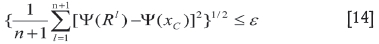
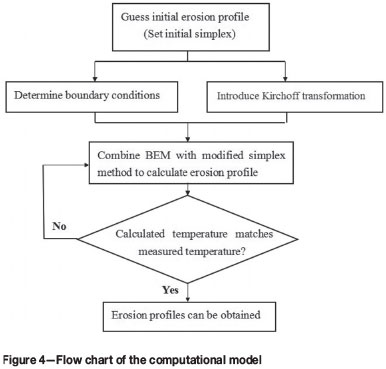
where ε is a convergence criterion, Rl is the element from the collection of 'simplex', and xc is the centroid (Nelder and Mead, 1965). The flow diagram of the computational model is shown in Figure 4. Since Equation [12] does not contain any domain integrals, only the boundary needs to be discretized. In addition, the solution of the Nelder-Mead simplex method (modified simplex method) does not need derivation to optimizing parameters, and this program would converge in a few minutes. Detailed information about BEM and the modified simplex method is given by Nelder and Mead (1965) and Kurpisz and Nowak (1995). The setting up of the mathematical model is described by Dong and Shaojun (2013).
Results
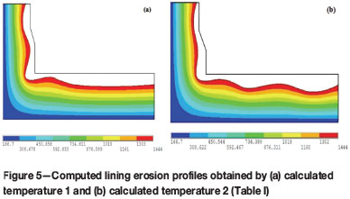
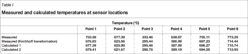
The average values of measured data from thermocouples 1-6 in Figure 2 were selected to calculate the erosion profile. Measured temperatures in domain Q also needed to be transferred by the Kirchhoff method (Table I). The computing methodology in Figure 4 was programmed in MATLAB (R2010a). The convergence criterion was chosen as 25 and the regularization term was defined as 0.015. More than one result could be acquired after the iterative convergence because of the diversity of the initial simplex and ill-posedness of the inverse problem. Two sets of calculated temperatures are illustrated in Table I. It can be seen that the difference between measured temperatures and calculated temperatures is less than 5°C, which indicates the effectiveness of the computing methodology developed. The corresponding erosion profiles from calculated temperature are shown in Figure 5. It can be seen that the calculated shapes of the inner profile vary widely, although the difference between two calculated temperatures is not obvious. In this case, it is preferable to introduce some other characteristics or industrial data for SAFs to validate the computing model and determine a reasonable solution.
Validation
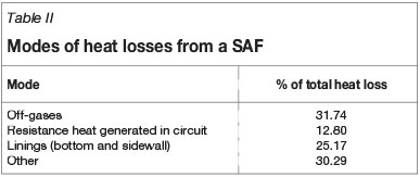
In previous work, Chu, Liu, and Wang (2009) assumed that an SAF is an adiabatic system and calculated its theoretical power consumption by material and energy balance theory. The results showed that the theoretical power consumption is 2713.46 kWh for producing one ton of FeNi (12%Ni) when the charge has been heated to 700°C. However, a real SAF is not an adiabatic system, hence it has a higher power consumption. According to investigations in an industrial plant, the actual power consumption is 3650 kW/t. A batch of FeNi is about 35 t and tap-to-tap time is around 4 hours. The modes of heat loss from a SAF have also been studied, and the heat losses through different paths are shown in Table II.
It is assumed that all these energies, which are generated by extra power consumption, are changed into heat. If the heat emissions from a SAF as indicated in Table II are correct, heat loss from the current SAF linings per unit time can be calculated as Equation [15]:
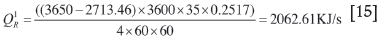
where  is the heat loss through the linings as calculated from the production data. Since the heat flux density of all boundaries in domain Ω can be calculated by virtue of BEM after erosion profiles have been obtained, the heat loss from the linings can also be calculated by integration. The computing process can be expressed as follows: since more than one vertical section, similar to domain Ω in Figure 2, was fitted with thermocouples to measure temperatures in a production SAF, several 3D solid lining models can be built by integrating to vertical sections; then the total heat loss of the linings can be calculated by summing the heat losses of all 3D models. The computational scheme, which takes one vertical section of domain Ω as an example, is illustrated in Figure 6.
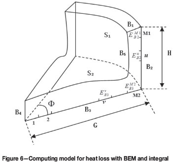
B4 in Figure 6 is assumed to be an axis located in the center of the SAF. One 3D model s generated by rotating the section around B4 through an angle  . Surfaces S1 and S2 are formed by the sweep of B2 and B3, with lengths of H and G, respectively. In addition, B2 and B3 in Figure 6 are discretized into some boundary elements, with the amounts of M1 and M2. The element on boundary B2, numbered as u, can be indicated by
  . Similarly, the vth element on boundary B3 is expressed as
  . Two surfaces can be formed by the sweep of elements
  and
and  , with heat fluxes of
  and
and  respectively, calculated by Equations [16] and [17].
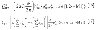
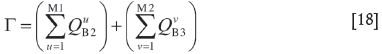
where h is the length of an element and q the heat flux density. It should be noted that the special parameter  in Equation [17] is equal to zero. The heat loss of the 3D model, denoted by r, is the sum of heat flux through S1 and S2, which can be calculated by Equation [18].
Six vertical sections were selected to arrange the thermocouples in the SAF, as shown in Table III. The positions of the sensors in each vertical sections were similar. Table III also shows three different calculated temperatures and the corresponding heat fluxes of 3D models per unit time, assuming three possible results for the erosion profile could be obtained in each section. Total heat loss of the lining per unit time could be calculated as follows:
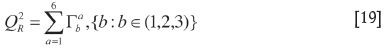
Where superscript a is the number of the vertical section, and subscript b is the possible number of calculated temperatures in vertical section a. Since three possible results for the erosion profile are obtained in each vertical section, the amount of possible  is equal to (
 )6. All computed results for
  need to be compared with
  . The optimal solution of
  is the value closest to
  .
.
An optimal calculated result for  is acquired after 729 comparisons, as illustrated in Equation [20]. The difference between optimal
  and
and  is 168.2 KJ/s.

In the process of calculating  , the SAF lining is supposed to be an ideal 3D solid that is similar to a cylinder, with tap-holes ignored. It should be noted that the temperature at the region near the tap-holes is higher. In the current model, the computed results for heat loss, ignoring the tap-holes, are lower than for a realistic situation. Erosion profiles obtained after validation could meet the requirements of temperature comparison method; furthermore, the calculated heat loss obtained by the current model approximates that computed with industrial data.
Conclusions
In order to monitor the erosion profile of the freeze lining in a SAF, a new two-step mathematical model was developed.
Kirchhoff transformation was applied in the first step to deal with the nonlinear partial differential equation, boundary conditions, and measured temperatures. The boundary element method was combined with the Nelder-Mead simplex optimization method in the second step to solve an inverse heat conduction problem using the measured data from thermocouples. The difference between calculated temperature and measured temperature is less than 5°C after the erosion profile is obtained.
The solutions are not unique owing to the differences of initial simplex and ill-posedness of inverse problems. The computational model was validated by comparison of heat losses from the lining. The heat release through the linings, which was calculated by BEM and integral calculus after the erosion profiles were obtained, could be computed using industrial data such as actual power consumption, tap-to-tap time, and output of ferronickel. The results showed that the difference in lining heat losses per unit time obtained by these two methods is around 168.2 KJ/s. The possible reason for this is that the tap-hole region is ignored in the model. A transient model and 3D lining model including the tap-hole will be developed in future work.
Acknowledgements
The authors gratefully acknowledge the financial support from National Natural Science Foundation of China (No.51274030) for this project. Our thanks to Mr Jichao Li from Ohio State University for useful discussions, and to Mr. Peixiao Liu from Sinosteel Jilin Electro-mechnical Equipment Co. Ltd providing valuable industrial data for the SAF.
Nomenclature
 Boundary element that is numbered as v on boundary B2, {v:v - (1,2...,M2)}
 Measured temperature of no. i thermocouple, {i: i - (1,2,3,4,5,6)}
 Length of element
 Calculated temperature at the location of no. i thermocouple, {i: i - (1,2,3,4,5,6)}
 Length of element
U Temperature transferred by Kirchhoff transformation
 Heat flux density of element
r Radial coordinates
 Heat flux density of element
z Axial coordinates
 Heat flux of the surface that is formed by the sweep of
  at an angle of
k thermal conductivity
 Heat flux of the surface that is formed by the sweep of
  at an angle of
Bo Boundary of domain Ω, {o: oa - (1,2,3,4,5)}
a Number of lining vertical section, {a: a- (1,2,3,4,5,6)}
f Temperatures function of boundary B2 and B3
b Number of calculated temperature in vertical section, {b: b - (1,2,3)}
g Temperatures function transferred from f by Kirchhoff transformation
n Amount of structure lines
A Structure point
M1 Amount of element on boundary B2
Lj Structure line, {j: j - (1,2,...n)}
M1 Amount of element on boundary B3
Pj Boundary point of B5, {j: j- (1,2,...n)}
Greek symbols
R1 Element from the collection of regular 'simplex' in modified simplex method, {l: l- (1,2,...n+1)}
αj Angles between B5 and structure line, {j: j- (1,2,...n)}
xC Centriod in modified simplex method
ε Convergence criteria
T* Fundamental solution in BEM
γ Regularization term
q* Derivative of  in BEM
Ω Computing region
C Integrating range
ψ Objective function
Φ Rotating angle of vertical section
H Length of B2 boundary
G Length of B3 boundary
 Heat release calculated with industrial data
 Heat release of 3D model formed by rotation of vertical section at an angle
 Heat release calculated by presented model
 Boundary element that is numbered as u on boundary B2, (u: u- (1,2,...,M1)}
References
Afshin, S. and Pawel, G. 2009. Non-destructive testing (NDT) and inspection of the blast furnace refractory lining by stress wave propagation technique. 5th International Congress on the Science and Technology of Ironmaking, Shanghai. pp. 951-955. [ Links ]
Akihiko, S., Hitoshi, N., Nariyuki, Y., Yoshifumi, M., and Masaru, M. 2003. Investigation of blast-furnace hearth sidewall erosion by core sample analysis and consideration of campaign operation. ISIJ International, vol. 43, no. 3. pp. 321-330. [ Links ]
Brànnbacka, J. AND Saxén, H. 2008. Model for fast computation of blast furnace hearth erosion and buildup profiles. Industrial and Engineering Chemistry Research, vol. 47, no. 20. pp. 7793-7801. [ Links ]
Carslaw, H. and Jaeger, J.C. 1959. Conduction of heat in solids. 2nd edn. Oxford University Press, Southampton. pp. 8-13. [ Links ]
Chu, S.J., Liu, P.X, and Wang, H.L. 2009. Calculation of theoretical power consumption and production cost of nickel ferroalloy. Ferro-Alloys, no. 4. pp. 1-7. [ Links ]
Dong, H. and Shaojun, C. 2013. Mathematical model for fast comptation of erosion profile in submerged arc furnace with freeze lining. 13th International Ferroalloys Congress Proceedings, Almaty, Kazakhstan. pp. 799-809. [ Links ]
Duncanson, P.L. and Toth, J.D. 2004. The truths and myths of freeze lining technology for submerged arc furnace. 10th International Ferroalloys Congress, Cape Town. pp. 488-499. [ Links ]
Karstein, S.I. and Skaar, M. 1999. Monitoring the wear-line of a melting furnace. 3rd International Conference on Inverse Problems in Engineering, Port Ludlow. pp. 1-11. [ Links ]
Kievit, A.D., Ganguly, S., Dennis, P., and Peietrs, T. 2004. Monitoring and control of furnace 1 freeze lining at Tasmanian electro-metallurgical company. 10th International Ferroalloys Congress, Cape Town. pp. 477-483. [ Links ]
Kouji, T., Takanobu, I., and Kouzo, T. 2001. Mathematical model for transient erosion process of blast furnace hearth. ISIJ International, vol. 41, no. 10. pp. 1139-1145. [ Links ]
Kuncan, Z., Zhi, W., and Xunliang L. 2009. Research status and development trend of numerical simulation on blast furnace lining erosion. ISIJ International, vol. 49, no. 9. pp. 1277-1282. [ Links ]
Kurpisz, K. and Nowak, A.J. 1995. Inverse thermal problems. Computational Mechanics Publications. pp. 53-65. [ Links ]
Lijun, W. and Huier, C. 2003. Mathematical model for on-line prediction of bottom and hearth of blast furnace by particular solution boundary element method. Applied Thermal Engineering, vol. 23, no. 16. pp. 2079-2087. [ Links ]
Nelder, J.A. and Mead, R. 1965. A simplex method for function minimization. The Computer Journal, vol. 7, no. 4. pp. 308-313. [ Links ]
Rodd, L., Voermann, N., and Stober, F. 2010. SNNC: a new ferro-nickel smelter in Korea. 12th International Ferroalloys Congress, Helsinki. pp. 698-700. [ Links ]
Surendra, K. 2005. Heat transfer analysis and estimation of refractory wear in an iron blast furnace hearth using finite element method. ISIJ International, vol. 45, no. 8. pp. 1123-1128. [ Links ]
Swartling, M., Sundelin, B., and Tilliander, A, and Jönsson, P.G. 2010. Heat transfer modelling of a blast furnace hearth. Steel Research International, vol. 81, no. 3. pp. 186-196. [ Links ]
Torrkulla, J. and Saxén, H. 2000. Model of the state of the blast furnace hearth. ISIJ International, vol. 40, no. 5. pp. 438-447. [ Links ]
Yu, Z. and Robit, D. 2008. Numerical analysis of blast furnace hearth inner profile by using CFD and heat transfer model for different time periods. International Journal of Heat and Mass Transfer, vol. 51, no. 1. pp. 186-197. [ Links ]
Zagaria, M., Dimastromatteo, V., and Colla, V. 2010. Monitoring erosion and skull profile in blast furnace hearth. Ironmaking and Steelmaking, vol. 37, no. 3. pp. 229-234. [ Links ]
Zhao H.B., Cheng S.S., and Zhao, M.G. 2007. Analysis of all-carbon brick bottom and ceramic cup synthetic hearth bottom. Journal of Iron and Steel Research International, vol. 14, no. 2. pp. 6-12. [ Links ]

