GENERAL PAPERS

 

Multi-mineral cut-off grade optimization by grid search

 

 

E. Cetin^I; P.A. Dowd^II

^IMining Engineering Department, Dicle University, Turkey
^IIFaculty of Engineering, Computer and Mathematical Sciences, University of Adelaide, Australia

 

 

---

ABSTRACT

Orebodies that contain more than one economically important mineral are generally evaluated by parametric cut-off grades. This approach often leads to mis-valuation of mineral deposits because cut-off grades are not based on the grades of each individual mineral and, because of the parametric formulation, are only indirectly related to the individual grade distributions. The only realistic approach is a formulation that accounts separately for each component mineral. The grid search method can be used as a means of multi-mineral cut-off grade optimization in this context.
This paper describes the use of the grid search method in cut-off grade optimization for multi-mineral deposits. The authors introduce the general concepts of the method and formulate its application to cut-off grade optimization; they describe a software implementation of the method that can accommodate cut-off grade optimization for mineral deposits that contain up to three economic minerals.

Keywords: cut-off grade, optimization, grid search, multi-mineral deposits.

---

 

 

Introduction

A cut-off grade for a mineral deposit is any grade that is used to classify the mineralized material for any required purpose. In the work reported here we take that purpose to be the classification of a mine's material as ore or waste, although the proposed approach is equally applicable to any other classification. Mineralized material above the cut-off grade is considered as ore and, subject to access constraints, can be mined, while material below the cut-off grade is considered as waste and, depending upon the mining method used, is either left in situ or sent to a waste dump.

Optimal cut-off grades are those that maximize some specified criterion such as profit or discounted profit. The determination of cut-off grades for a single-mineral deposit is relatively simple. However, for multi-mineral deposits the determination of cut-off grades is a more complex process.

Multi-mineral deposits in which the constituent minerals are positively correlated, and therefore tend to be co-located, are generally valued, planned, and operated on the basis of parametric, or equivalent, cut-off grades. The use of equivalent grades for these types of deposits has been standard practice in the mining industry for many years, especially for base metal deposits. In this approach, each mineral is converted to its equivalent economic value in terms of one of the minerals, which is taken as a standard. For example, in a silver-lead-zinc deposit a weighted sum of the three metal grades may be used to provide a single lead-equivalent grade. This is generally done to avoid the complexities of a three-dimensional (or, in general, n-dimensional) grade analysis. It is also done because the constituent minerals are largely co-located; in stratiform silver-lead-zinc deposits, for example, correlation coefficients among the three variables usually range from 75% to 90%. After combining the individual mineral values into a single equivalent value, the optimum cut-off grades for the equivalent variable can be found by using any of the established methods of single mineral cut-off grade optimization, e.g., Lane (1964, 1988), Dowd (1976). Operating cut-off grades for the equivalent grades do not necessarily correspond to achievable, or even meaningful, cut-off grades for the grade-tonnage distributions of the individual minerals. Perhaps more importantly, except for cases in which the component minerals are very highly correlated, an optimal schedule based on equivalent cut-off grades may differ significantly from a truly optimal schedule that adequately accounts for all of the component minerals. While there is a direct relationship between the individual grades and the equivalent grade, there is no unique inverse relationship from the equivalent grade back to the individual grades. In the mining process, the equivalent cut-off grades are only Multi-mineral cut-off grade optimization by grid search indirectly related to the grade distributions of the component minerals. The amounts of each mineral extracted in the mining stage and sent to the processing plant and subsequent stages are estimated on the basis of equivalents and not on the basis of the component minerals. Thus, the actual amounts of each individual mineral above the equivalent cutoff grade will differ from the values calculated from the equivalents, and this difference will increase as the correlation among the components decreases. Since actual production of individual minerals cannot be determined from the equivalents, it is not possible to generate accurate individual mineral recoveries or financial outcomes. Thus, using equivalent grades may undervalue or overvalue mining projects.

In the context of Lane's (1964, 1988) staged approach to cut-off grade theory, the procedure may be valid if there are no constraints on the stages that follow the extraction, or mining, stage. If, however, one or more of the minerals is subject to subsequent stage limitations, the process is not valid. For example, if there is a refinery/market limitation on one mineral, then excess production of that mineral cannot be sold and, as a result, the mineral cannot be valued on the basis of the contract price. Hence, the influence of the capacities of the mineral processing plant and the refinery/market stages invalidates the parametric cut-off grade approach and, therefore, necessitates individual accommodation of each mineral.

The objective of the work described in this paper is to find a feasible method of determining optimal production sequences of cut-off grades without using the equivalent, or parametric, cut-off grades.

The main contribution of this work to cut-off grade optimization is to extend Lane's grid search method to accommodate more than two minerals. Our method for selecting the grid points differs from that of Lane and gives better results by significantly increasing the search area. We show that our method can readily accommodate optimizations of up to five constituent minerals.

 

Optimization of cut-off grades for multi-mineral deposits by the grid search method

The grid search method is based on the concept of dividing the search area into equal size grids and searching for the optimum among the grid points. The method involves setting up a suitable grid in the design space, evaluating the objective function at all grid points, and finding the grid point corresponding to the optimum value, i.e., minimum or maximum value (Rao, 2009). Lane (1988) was the first to propose the technique for optimizing the time sequence of cut-off grades for two-mineral deposits. The grid search method proposed by Lane can be applied to mineral deposits that contain more than two mined minerals by adding a stage to the calculations for each mineral; the process does, however, become more time-consuming as the number of minerals increases.

Lane (1988) proposed a form of the grid search technique that involves calculating the net present values for four different limiting cut-off grades. The ore/material ratios (i.e., the ratio of the amount of ore to the total amount of mineralized material in the deposit) and average grades for each pair of cut-off grades can be calculated from the grade distributions. Net present values can then be calculated for a limited mining rate (vm), a limited processing rate (vh), a limited refinery/marketing rate (vk1) for the first mineral, and a limited refinery/marketing rate (vk2) for the second mineral. The controlling capacity for each pair of cut-off grades is the one that corresponds to the least of the four net present values calculated. It is this figure that has to be maximized among the different pairs of cut-off grades in order to find the optimum pair.

The main advantage of the grid search method over the equivalents method is that it is more general, i.e. the equivalents method is applicable only when there is a strong positive correlation among the constituent minerals. The grid search method can be applied even when the secondary minerals are of minor importance.

Lane (1988) suggested using a primary grid of 9 x 9 cells, which yields 100 grid points. As a second step, he proposed a secondary grid of 6 x 6 cells, which yields 49 grid points, covering the four original cells that surround the maximum point. Finally, a third grid of 6 x 6 cells covering the four cells that surround the maximum point in the secondary grid was proposed. As a safeguard, Lane also suggested that, if the maximum occurs on the boundary of the second or the third grid, the grid should be relocated around the nearest point with no change in scale. This process ensures that the maximum will be found even when it is on a steep ridge between grid points. The process involves the calculation of 198 grid points.

Lane (1988) claimed that the process of using three subsequent grids gives an accuracy of one in 9 x 3 x 3 - in other words, 1 in 81, which is close to 1%. In fact, there is no obvious proof or evidence that using three subsequent grids, instead of one, improves the search process. The optimum point is not necessarily near the maximum point in the first grid and, by discarding the search area outside the four cells around the maximum point in the first grid, there is a danger of missing the global optimum target.

Mohammed (1997) applied Lane's grid search method to a copper and gold deposit. He used the grid selection method suggested by Lane and developed a computer program for mineral deposits that contain two economic minerals. He assigned the grade intervals for a given grade-tonnage distribution as grid points for the primary grid. The application of the method to a sample deposit yields pairs of cut-off grades that are in decreasing order.

Ataei and Osanloo (2004) used the grid search method together with genetic algorithms to determine optimum cutoff grades for multiple metal deposits. They limited the use of the grid search method to searching for upper and lower limits of the constituent minerals in grade-tonnage tables. They then used genetic algorithms to search for the optimum in detail.

For orebodies that contain more than two minerals, the grid search method is still useful. For an orebody with three economic minerals, there will be five operational stages that restrict the throughput, the fifth one being the refinery/marketing limiting stage for the third mineral. As a result, there are five different net present values representing each of the stages. Although the grade-tonnage distribution is three-dimensional the approach is not very different to the two-mineral case. The computing time, however, increases significantly with the inclusion of each additional mineral.

The following expressions are derived for the calculations used in the grid search method for mineral deposits containing three mineable minerals.

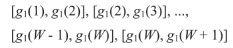
Assume that the grade-tonnage distribution of a mineral deposit consists of W grade cells for mineral 1. Hence, there would be W + 1 grade limits. The representation of the corresponding grade for the different cells would be:

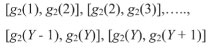
As there is more than one mineral in the grade distribution, the deposit will have W number of grade distributions for mineral 2. Assume that each of the grade distributions for mineral 2 have Y individual cells. As a result, there would be Y + 1 grade limits. The representation of the corresponding grade for different cells would be:

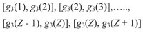
As there are three minerals in the grade distribution, the deposit will have W x Y number of grade distributions for mineral 3. Assume that each of the grade distributions for mineral 3 has Z individual cells. As a result, there would be Z + 1 grade limits. The representation of the corresponding grade for different cells would be:

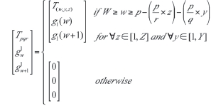
Let:

 the lower grade limit g(w) for a given cell [g(w), g(w + 1)] be the cut-off grade of mineral 1 representing interval p

 the lower grade limit g(y) for a given cell [g(y), g(y + 1)] be the cut-off grade of mineral 2 representing interval q

 the lower grade limit g(z) for a given cell [g(z), g(z + 1)] be the cut-off grade of mineral 3 representing interval r.

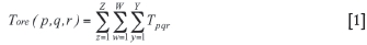
then the amount of material above the cut-off grade, the amount of the material below the cut-off grade, the average grade of mineral 1 above the cut-off grade, the average grade of mineral 2 above the cut-off grade, and the average grade of mineral 3 above the cut-off grade can be found by using the following equations:

where

where:

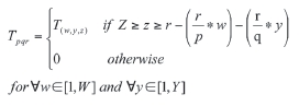
T_ore(p,q,r)    is the amount of material above the cut-off grade for the pth and qth and rth grade intervals

T(w,y,z)    is the amount of material for the given grade limits

p    is the grade interval for the first mineral

q    is the grade interval for the second mineral

r    is the grade interval for the third mineral.

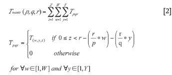
where:

T_waste (p,q,r)   is the amount of material below the cut-off grade for the pth and qth and rth grade intervals.

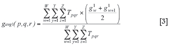
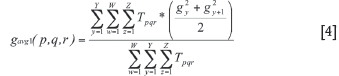
where:

g_avg1 (p,q,r)   is the average grade of the first mineral above the cut-off grade for the pth grade interval of the first mineral and the qth grade interval of the second mineral, and the rth grade interval of the third mineral

g₁(w)   is the lower grade limit of a given cell for the first mineral

g₁(w + 1)   is the upper grade limit of a given cell for the first mineral.

where:

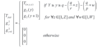
g_avg2 (p,q,r)   is the average grade of the second mineral above the cut-off grade for the pth grade interval of the first mineral and the qth grade interval of the second mineral, and the rth grade interval of the third mineral

g₂(y)    is the lower grade limit of a given cell for the second mineral

g₂(y + 1)    is the upper grade limit of a given cell for the second mineral.

where:

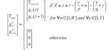
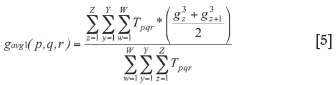
gavg3(p,q,r)    is the average grade of the third mineral above the cut-off grade for the pth grade interval of the first mineral and the qth grade interval of the second mineral, and the rth grade interval of the third mineral

g3(z)   is the lower grade limit of a given cell for the third mineral

g3(z + 1)    is the upper grade limit of a given cell for the third mineral.

The ore/material ratio can be calculated from Equation [6].

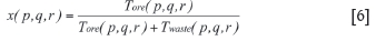
where:

x(pq,r)    is the ore/material ratio for the pth grade interval of the first mineral and the qth grade interval of the second mineral.

The average grades and the ore/material ratio values that were generated by these equations are for the grade intervals of the specified grade-tonnage distribution. If the grade intervals are chosen as grid points, the net present values for the five different limiting stages can be calculated by using the equations given below. However, if the grid points are assigned explicitly, the corresponding net present values for the grid points, the values of the ore/material ratio, and the average grades of each of the three minerals above the cut-off grades for each grid point are found by interpolation. Once these values for the grid points representing any pair of cutoff grade points have been found, the net present values for the five different limiting stages can be calculated by using the following equations.

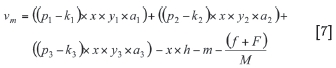
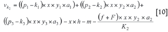
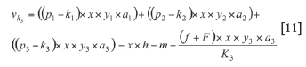
where;

p₁   is the price of the first mineral per unit of product

p₂    is the price of the second mineral per unit of product

k₁    is the marketing variable cost of the first mineral

k₂    is the marketing variable cost of the second mineral

x    is the ore / material ratio

y₁    is the yield of the first mineral during treatment (recovery)

y₂    is the yield of the second mineral during treatment (recovery)

a₁    is the average grade of the first mineral

a₂    is the average grade of the second mineral

h    is the mineral processing variable cost

m    is the mining variable cost

f    is the fixed cost

F    is the opportunity cost

t    is the time unit of resource

vm    is the net present value for a limited mining rate

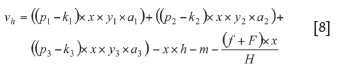
vh    is the net present value for a limited mineral processing rate

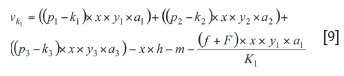
vk₁    is the net present value for a limited refinery/marketing rate for the first mineral

vk₁    is the net present value for a limited refinery/marketing rate for the second mineral

vk₁    is the net present value for a limited refinery/marketing rate for the third mineral

y₁    is the yield of the first mineral during treatment (recovery)

y₂    is the yield of the second mineral during treatment (recovery),

y₃    is the yield of the third mineral during treatment (recovery)

a₁    is the average grade of the first mineral

a₂    is the average grade of the second mineral

a₃    is the average grade of the third mineral

K₁    is the maximum refinery or marketing capacity for the first mineral,

K₂    is the maximum refinery or marketing capacity for the second mineral

K₃    is the maximum refinery or marketing capacity for the third mineral.

After deciding on the net present values for each stage, the highest possible net present value is found as:

As five stages restrict the process, for any grid point, the minimum among the five values gives the maximum possible present value and the maximum among them gives the optimum grid point. The cut-off grades that lie on the optimum grid point give the optimum cut-off grades for three minerals.

The grid search described here is based on Lane's grid search method but with some significant differences. The main difference is the size, and method of selection, of the grid: only one grid is assigned instead of three. The selection of grid points in the grid is done explicitly, rather than using the grade intervals for the given grade-tonnage distribution. More grid points have been used in the work described here than were used by Lane (1988).

Lane (1988) proposed a primary grid of 9 x 9 cells, a secondary grid of 6 x 6 cells and a third grid of another 6 x 6 cells. The process involves calculation of only 198 grid points. Lane claimed that the process of having three subsequent grids gives an accuracy of 1 in 81. However, there is no obvious proof that using three subsequent grids improves the search process. In any case, due to the significant increases in computer memory capacity and computational speed, it is now possible to search a finer grid, which has a better coverage than the method of grid selection suggested by Lane. As a result, far more grid points can be searched for the optimum than in Lane's method. For the case of two minerals, a grid of 100 x 100 cells, yielding a total of 10 201 grid points, can be searched. The number of grid points is not fixed but rather left to the user of the program.

 

Case studies

Two case studies have been included here to illustrate the application of the software for determining optimum cut-off grades.

Case study 1

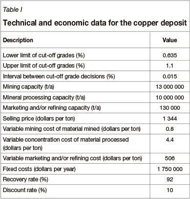
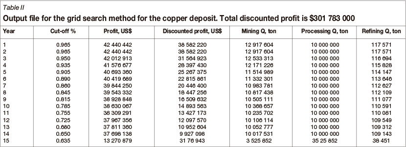
Case study 1 is a copper deposit. The grade-tonnage distribution for the deposit is shown in Figure 1 and the technical and economic data is given in Table I. The results showing the complete cut-off grade schedule are given in Table II.

 

 

 

 

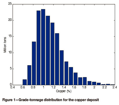
A total of 32 different cut-off grades were searched for the optimum. The mining operation terminates in 14.35 years and total production is 143 525 852 tons. Total discounted profit is $301 783 000.

The cut-off grades, and as a result the depletion rates, are lowered progressively throughout the life of the mine. Cut-off grades begin at 0.965% and end at 0.635% in less than 15 years.

To verify the results generated by the software, the data for case study 1 was processed by the MINVEST software package (Dowd and Xu, 2000). The same data used for the grid search method, given in Table I, was entered and Lane's method of limiting and balancing cut-off grades (Lane, 1964, 1988) was selected from the package to generate a solution. The results were substantially similar to the production schedule given in Table II. The results obtained from MINVEST are given in Table III and can be compared with the grid search method results given in Table II. Some improvements in total discounted profit (0.03%) is achieved, that can be seen by comparing the total discounted profits of the tables (Table II and Table III). This exercise demonstrates the robustness of the method used in this paper.

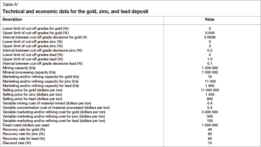
Case Study 2

Case study 2 is a gold, zinc, and lead deposit. The technical and economic data are given in Table IV and the results are given in Table V.

Sixteen different cut-off grades for each mineral were searched for the optimum. The optimum schedule terminates in 8.07 years with a total production of 8 066 991 tons. Total discounted profit is $439 100 000.

The cut-off grades, and as a result the depletion rates, are lowered progressively throughout the life of the mine.

Although a maximum net present value requires a decreasing cut-off grade schedule (Lane, 1964; Dowd, 1976; Cetin and Dowd, 2002), in the case of multi-mineral deposits, the decreasing cut-off grade may not apply uniformly to each mineral. In Table V, for example, the cut-off grade for lead in the ninth year increases, and such variations are more likely as the correlation among the component minerals decreases and the difference in the financial values of the components increases.

 

Conclusions

Optimization of cut-off grades for multi-mineral deposits is generally done by means of parametric, or equivalent, cut-off grades. Although this approach simplifies the optimization process, it may not achieve a true optimum, especially for orebodies in which there is not a highly significant positive correlation among the component minerals. The objective of the work described in this paper is to find the best method of determining optimal production sequences of cut-off grades without using the equivalent, or parametric, cut-off grades. A complete, detailed mine production schedule that includes mining and other access constraints is beyond the scope of this work. For this reason no mining or other access constraints are included in the formulation of the problem. The orebody is completely defined by grade-tonnage distributions and it is assumed that any parcels of ore selected for production have the same characteristics as the specified grade-tonnage curves and are immediately accessible.

Although the work described here is not restricted to open-pit mines, the computer program developed is more suitable to open-pit mining operations than to underground mines. In underground mines a greater proportion of waste is left in situ and access constraints are simultaneously more restrictive and less comprehensive than in open pits. In this study, variable mining costs are applied to a depletion rate, which means that all the material required to achieve a specific tonnage and grade is effectively excavated regardless of whether it is processed.

The computer program is based on the grid search method. The method has previously been applied to two-mineral deposits. The work described here extends the grid search method to mineral deposits that contain up to three mined minerals. The grid search method described here is based on Lane's grid search method but with some important differences in the size, and the method of selection, of the grid.

The work described in this paper is the first application of the grid search method to three-mineral deposits.

 

References

Ataei, M. and Osanloo, M. 2004. Using a combination of genetic algorithm and the grig search method to determine optimum cutoff grades of multiple metal deposits, International Journal of Surface Mining, Reclamation and Environment, vol. 18, no. 1. pp 60-78.         [ Links ]

Cetin, E. and Dowd, P.A. 2002. The use of genetic algorithms for multiple cutoff grade optimisation. Proceedings of the 30th Symposium on Applications of Computer and Operations Research in the Mineral Industry (APCOM2002), Littleton, Colorado, USA. pp. 769-779.         [ Links ]

Dowd P.A. 1976. Application of dynamic and stochastic programming to optimise cut-off grades and production rates. Transactions of the Institution of Mining and Metallurgy Section A: Mining Industry, vol. 81. pp. 160-179.         [ Links ]

Dowd, P.A. and Xu, C. 2000. MINVEST User's Manual. Computer Aided Mine Design Centre, University of Leeds. 272 pp. [now available from the authors at the University of Adelaide, Australia: peter.dowd@adelaide.edu.au].         [ Links ]

Lane, K.F. 1964. Choosing the optimum cut-off grade. Colorado School of Mines Quarterly, vol. 59, no 4. pp. 811-829.         [ Links ]

Lane, K.F. 1988. The Economic Definition of Ore. Mining Journal Books, London, UK.         [ Links ]

Mohammed, W.A.A. 1997. Multi-mineral cut-off grade optimization with option to stockpile. Master of Science thesis, Colorado School of Mines.         [ Links ]

Rao, S.S. 2009. Engineering Optimization: Theory and Practice. John Wiley & Sons, Chichester, UK.         [ Links ]

 

 

Paper received Apr. 2012
Revised paper received Jul. 2013

 

 

© The Southern African Institute of Mining and Metallurgy, 2013. ISSN 2225-6253.