GENERAL PAPERS

 

A real options application to manage risk related to intrinsic variables of a mine plan: a case study on Chuquicamata Underground Mine Project

 

 

J. Botin; M.F. Del Castillo; R. Guzman

Pontificia University, Católica de Chile, Santiago, Chile

 

 

---

ABSTRACT

Traditional risk quantification methods provide little information on the sources of risk, and tend to produce static over-conservative evaluations, which do not account for changes in the performance of the project. Capital investment decisions for large mining projects require more complex risk evaluation models that include the value of flexibility and the different risk levels associated with uncertainty on project variables (price, grade, dilution, and production rates, among many other). In this context, real option valuation (ROV) methods have proven potential to quantify the risk associated with such variables and integrate alternative scenarios and management strategies into the evaluation process. In this paper, a risk quantification model is developed that successfully quantifies the risk associated with dilution, as a function of production rate. This model is then validated in a case study on the Chuquicamata Underground Mine project.

Keywords: real options, risk management, risk quantification, dilution, minine planning.

---

 

 

Introduction

Unlike most other industries, in mining, the 'raw material' (ore) is not a commercial product for which the buyer knows the exact composition and properties, but a natural material. Its chemical composition and physical properties must be estimated from sampling, laboratory testing, and expert judgment (Maybee, B., Lowen, S., and Dunn, P. 2010). Moreover, tonnage and unit value of ore resources vary with price and other market parameters. This fact explains why the orebody is one of the main sources of risk in a mining business (Sayadi, A., Heidari, S., and Saydam, S. 2010; Rozman, L.I. 1998).

Because of this uncertainty and variability with time, capital investment decisions cannot rely on static parametric evaluations, such as discounted cash flow (DCF), as these methods provide only a picture of the value of a project associated to a 'base case' scenario, but fail to consider the dynamic character of decision-making over the life of the project.

Real options valuation (ROV) represents a better approximation to the way an investor sees a project: accepting uncertainty and focusing on the potential project responses to the range of possible future conditions. These 'future conditions' include internal (technical) as well as external (market) variability (Amram, M. and Kulatilaka, N. 1999).

Current applications of ROV focus mainly on external variables, such as commodity price and exchange rate, which are controlled by external factors and cannot be engineered. This study focuses on real options (RO) as a tool for quantifying and managing the risk associated with the variability of technical mine planning parameters, internal variables which are characteristic to every project.

 

Risk valuation

Traditional vs. real options approach

Conventionally, the DCF method is used to evaluate projects where parameters are estimated at a fixed 'most likely' value, and risk analysis is limited to scenario and sensitivity analyses(Samis, M., et al., 2011; Torries, T. 1998; Whittle, G., Stange, W., and Hanson, N. 2007). Although this method does deliver an indication of the project's NPV, it doesn't account for real variability, nor does it provide management with guidance on the different sources of uncertainty and their likelihood.

ROV methods were developed as an extension of financial options derivatives to tangible investment projects. An option -financial or real - is a right, but not an obligation, to perform an act for a certain cost, at or within a period of time. In this context, ROV focuses on adding value to the project by taking advantage of uncertain situations, gaining from favourable scenarios, and hedging from downside risks ( Dimitrakopoulos, R., Martinez, L., and Ramazan, S. 2007; Martinez, L. and McKibben, J. 2010).

However, it is important to state that ROV is not a substitute for the conventional DCF method, but rather a complement that adds the capability of capturing the value associated with management reacting to change. Focusing on this concept, Dimitrakopoulos and Sabour (2007) and Sabour and Wood (2009) stated that a key advantage of ROV is the ability to incorporate the value of management reacting on the basis on new information. The method provides a transparent guideline for analysing the timing of strategic and operational decisions, as it deals with the different sources of uncertainty individually.

Options 'on' vs. options 'in' projects

Most ROV applications focus on risk associated with market uncertainties, a research field where RO methods have made a significant contribution. However, examples of the application of RO in the valuation of internal uncertainties are scarce. In this regard, Wang and de Neufville (n.d.) define the concept of options 'on' projects as the options that analyse variables that act upon the project (external conditions), and options 'in' projects as options that have the potential to actually change the design of the system.

In this research line, some authors have applied 'in-project' ROV to evaluate compound risk from extrinsic and intrinsic variables. Dimitrakopoulos, Martines, and Ramazan (2007) use RO models that combine price and geological variables in order to manage risk associated with grade uncertainty and use a 'minimum acceptable return on investment' as the evaluation criteria. Akbari et al. (2009) use a binomial tree to simulate the metal price, and define the optimal starting point of the mine and the ultimate pit limit dependent on 'today's price. Maybee et al. (2009) compare the DCF method with ROV to quantify the value of flexible development strategies in a block caving and cut and fill mine, by using a traditional replicated portfolio to account for price uncertainty.

Very few authors have applied ROV to evaluate risk from purely intrinsic variables. It is worth highlighting the work of Kazakidis and Scoble (2003), who studied the application of RO to analyse three 'in-the-project' option scenarios on ground-related problems: first, a sequencing option for increasing the flexibility of the production plan; secondly, the option of hiring extra rehabilitation crew to deal with ground-related problems; and thirdly, a trade-off study between different flexible alternatives in order to optimize the mine plan. The decision is made by using two parameters: a 'flexibility index' (also used by Musingwini et al. 2007) and the capital cost of each option considered (the option's price). This is a very good example of RO applications 'in' projects, where the focus is placed on increasing project flexibility.

It becomes evident that, despite the great potential of ROV application 'in-the-project' variables, references on the subject are scarce. The research described in this paper deals with the application of 'in-the-project' ROV to manage risk associated with production rate, grade dilution, and other mine planning variables.

The literature describes several limitations referring to the use of conventional DCF valuation of mining projects. First, variables are assigned a constant value, not considering their stochastic reality (Reichmann, W.J. 1962). A second limitation is that the DCF approach assumes that investment decisions are made 'now or never', without considering the value of strategy and management (Cardin, M.A., de Neufville, R., and Kasakidis, V. 2008). A third shortcoming is that the DCF method tends to undervalue projects by not considering management options and other scenarios alternative to the 'base case'. In fact, during the operational stages of a project, management has the capacity to react to the variation of a parameter by making decisions that would minimize negative outcomes and take advantage of the positive, similarly to what ROV considers. In many cases, management reactions can be predicted and considered as real options at feasibility decision stages. Traditional DCF neglects the value added associated with future management reaction to change and, therefore, it may lead to wrong feasibility decisions. The challenge is to design a system that can cope with different future scenarios by means of in-built flexibility, thus allowing management to adapt (De Neufville, R. and Scholtes, S. 2011). ROV provides the tools to integrate flexibility into the initial model, thus increasing its reliability.

 

Risk management model

Risk management may be defined as the act or practice of dealing with risk (Kerzner, 2013). The goal of this process is to acquire an understanding of the project's possible outputs for taking decisions that will maximize the project's value. Botín et al. (2011) present a 2-D impact-likelihood model for risks acting on a capital investment project (Figure 1), which results in four types of risks: fatal flaws (A), manageable risks (B), catastrophic risks (C), and bearable risks (D).

 

 

A risk management flow model is developed using this classification (Figure 1). Its goal is to define the actions that must be taken to manage each type of risk. In this flow chart, high impact risks (A and C) must be eliminated during the engineering stages of the project. On the contrary, type D risks are not considered in the analysis, as the cost of managing them is higher than the maximum possible gain obtained by eliminating them, and thus they must be accepted as 'bearable'.

Figure 2 presents a simplified value chain of the project evaluation processes. In this context, type B risks (Figure 1b) can be grouped in two types: (i) risks that can be managed within the process in which they originated, and hence do not have an impact in processes downstream, and (ii) risks that cannot be managed in a single process and hence may impact downstream processes in the value chain. An example of the first type is the risk associated with ore hardness, a risk pertaining to the process of 'mineral processing engineering' (Figure 2). Here, a higher-than-expected hardness would reduce milling rates. This impact can be managed within the mineral processing scenario by selecting a larger mill. An example of the second type is the risk associated with ore grade and dilution. In this case, the risk from a higher-than-expected grade/dilution, originated within the 'mine planning' process (Figure 2), would impact all processes downstream and, as shown in Figure 1b, may be evaluated and managed by using ROV.

 

 

The real option

This study focuses on type B (i.e. economically manageable) risks, particularly risks associated with grade dilution, a key parameter in the mine planning process. In fact, a higher-than-expected grade dilution would also impact on the mill design and engineering process and all processes downstream 'mine planning' in the lifecycle (Figure 2). It is worth noting that the model will stay independent from external variables (market conditions), focusing solely on the internal/technical variability of mine dilution.

In this paper, ROV is applied to evaluate dilution risk using a real option on an increased production capacity of the mine-mill system, allowing it to process the extra waste rock resulting from a higher dilution, thus enabling metal throughput to be sustained when dilution is higher than planned.

Obviously, an increase in operating capacity incurs extra costs, both operational and capital. This cost structure resembles that of a financial option derivative, where the capex is the premium paid to 'buy' the option of acquiring extra system capacity (cost of having an option in the future), and the opex is the exercise cost, paid only if the option is executed.

Case study: Chuquicamata Underground Mine project

This case study analyses the Chuquicamata Underground Mine project, owned by Codelco. Chuquicamata has been operating as an open pit since 1915, and is now planning to go underground, as a four-panel macro-block caving operation. The project is based on a production rate of 140 kt/d, over 40 years (with a 6-year ramp-up, a 5-year ramp-down, and 29 years of steady production at maximum capacity (Ovalle, 2012), plus almost 10 years of initial development, which makes this project one of the largest underground operations in the world.

The sales data, as well as all other base-case deposit information such as the ore grade, dilution, and total reserves, are summarized in Table I. Sustaining capital and maintenance costs, as well as closing expenses, are all included in the capex value, calculated as the net present value of all the costs. With this data, an annual cash flow is developed, which presents a NPV of US$1875 million, with an 8% discount rate, and is summarized in Table II. Together with this, a detail of the annual total and net cash flows for the life of mine (LOM) are presented in Figure 3. In this current project, the initial investments started in year 2004 with the development, and the actual costs were considered for the NPV calculation. It can also be noted that there is negative cash flow in the last years. This is due to closing costs, and because of the heavy punishment of the DCF method over long projects, the last years have very little influence over the cumulative NPV.

 

 

 

 

 

 

As presented in Table II, a 57% tax is applied over the revenue after depreciation (for simplicity, a 5-year linear depreciation was considered). This high percentage is due to the fact that Codelco is a state company. Also, no income or expense from the open pit operation was considered in this cash flow, as Codelco treats both operations as separate projects. This scenario will be used as a base case to compare the future options' performance.

Cost of flexibility

To calculate the extra capex of the expanded operation, the Williams' model may be used as a cost estimating method. The Williams's model or Williams' rule is based on a cost relationship that exists between two plants or equipment of different capacity, power, or volume, but of similar characteristics. In general, Williams' rule is valid only for an 'order of magnitude' estimate but when used to estimate the capex for the same system at two different production rates, it provides the necessary accuracy. This formula may be expressed as:

where r = plant's expansion weight factor

In this case, C_B and C_A are respectively the capex for the base case and the expanded system capacity, and a Williams' exponent 'm' of 0.7 is used (Mular, A.L. 2002). The main difficulty of this quantification is to determine the appropriate weight factor: the one that hedges the risk derived from dilution's uncertainty without over-dimensioning. To do this, we first must understand how dilution will behave once the mine is in operation. This is explained in the following sections.

Modelling dilution in block caving

In this case study, the model used to simulate the ore-waste mixing process corresponds to a volumetric model developed by Laubscher (Diering, J.A. and Laubscher, D.H. 1988; Hudson, J.A., 1993).

The model is based on one linear parameter: the percentage of dilution entrance (PDE), which represents the percentage of the column that has to be drawn before waste material is perceived at the drawpoint of the block-cave. Correspondingly, as the model's output is a linear mixture along the column, there is a line that represents the waste material that crosses the column's centre at exactly its midpoint. Extrapolating this relation, dilution may be expressed in terms of the PDE:

For the base case of this case study, PDE is 50% for the first level and 40% for the following three levels, which results in dilutions of 12.5% and 15% respectively.

Dilution variability

The Laubscher model assumes that ore geometry and mechanical behaviour are constant, which is an oversimplification. Because of this, the in situ and the diluted block models produced by the Laubscher method will be used to develop a stochastic function that represents the dilution uncertainty.

This gradual grade reduction is the source of uncertainty. The actual PDE value is unknown and variable for each draw, therefore dilution does not occur linearly as the model proposes. This effect is presented in Figure 4, where the left image shows the ore-waste contact line, and the right image shows the resulting orebody after the mixing process of a 40% PDE.

 

 

Furthermore, the Laubscher model acts only vertically over the column, without considering sloping or horizontal flows of waste (here referred to as 'horizontal dilution').

The variability of 'ore grade' may be expressed as a distribution function, which is modelled from a histogram of block model grades (diluted and undiluted), by calculating the percentile variability comparing by range the grades of the original in situ model (left of Figure 4), with the diluted model from Laubscher's simulation (right of Figure 4). This data is then used to create a new histogram representing the probability of dilution per block. This procedure not only allows determining the most probable dilution values, but it also shows the complete behaviour of the variable. The sample presents a mean of 20.6% dilution, and a standard deviation of 19.5%.

The dilution model was developed by fitting the data of this histogram into the Arena Software^a (student edition), and running the input analysis tool. The best fit was obtained with the lognormal function in Figure 5. With a square error of 1.07%, it makes a robust model for dilution.

 

 

Horizontal dilution

The Laubcher model does not account for the dilution from adjacent columns and, more importantly, from the host rock at the boundaries of the orebody (White, 1990). This secondary dilution is denoted as 'horizontal dilution', and correspondingly, the previous model will be called 'vertical dilution'.

As the focus of this study is on long-term planning (yearly basis), the exact dilution of each column is not relevant. Therefore, in the estimation of 'horizontal dilution' only the host rock waste is considered, and is assigned a constant grade of 0.1% Cu, 20 ppm Mo, and 0.003% As.

Figure 6 represents a geometrical model of gravitational flow of waste material from host rock into the ore columns. Here, R is the radius of the gravitational ellipsoid of a given extraction column and R_i = R ^. (1+w_z) the interaction radius of a drawpoint, where w_z represents a weighting factor the value of which depends of the rock quality of zone z. The horizontal flow is represented by the dotted lines, and at boundary drawpoints it corresponds to waste material from host rock (traced area in Figure 6). For simplification purposes, this area may be calculated as the area of the right-angled triangle created by the column's height (H_C), and the interaction radius (R_i).

 

 

To calculate the tonnage of waste rock entering the operation as dilution, the simplified traced area (variable due to rock quality by zone) is multiplied by each level's external perimeter (also differentiated by zone) to obtain the total volume of waste material surrounding the deposit (which has the potential to enter the drawbells), and then multiplied by the host rock density (d_w = 2.57 t/m³). Knowing the dimensions of each macro-block, and of the pillars left between them, each level's perimeter is calculated.

The orebody is classified into three zones according to geology and geotechnical conditions. Each zone is characterized by a value of the subsidence angle, provided by Codelco. In the base case, an average subsidence angle of 50° was assumed for the entire orebody. As the braking angle is inversely proportional to the column's resultant radius, the weighting factor (w_z) for each zone (i) is calculated as the relative difference between the breaking angle value of the zone (a_í) and the base case angle (a_BC = 50°), as shown in Equation [3] (note that a lower angle means poorer rock quality, causing more rock flow and bigger affected radius).

As presented in the extraction grid in Figure 6, Chuquicamata's mine design defines a distance between drawpoints (circled dots) of about 35 m x16 m. This figure represents the extraction details of a macro-block, and according to the deposit's orientation, the host rock is located to the east and west of this macro-block. Because of this, the dilution radius corresponds to the oblique distance presented by R_BC in Figure 7, which by projecting the ellipsoids created by the interaction zone (Figure 6), has a length of approximately 9 m.

 

 

With this information, the value of each radius is calculated by dividing the base radius (9 m) by the weighting factor for each zone, as summarized in Table III.

 

 

Finally, to calculate the horizontal dilution (D_H), the total waste tonnage (integrated by zone and level) is divided by the total extractable tonnage (mineral + dilution), obtaining a value of 5.1%:

where

i = Deposit's zone. 1: west, 2: north-east, 3: south-east

j = Mine level, from 1 (top) to 4 (lowest bottom)

P_ij = Perimeter of zone j on level i (m)

R_i = Average radius of zone i (m)

H_j = Column height of level j (274, 235, 237, and 235 m)

d_w = Waste rock density (2.57 t/m³)

t_T = Total extractable tonnage (1581Mt)

As shown in the left image of Figure 7, every macro-block of the Chuquicamata Mine is in contact with the host rock, and at least two macro-blocks are extracted each year. Because of this, the horizontal dilution can be added homogeneously to the whole mine plan.

The dilution model

As described previously, dilution has two components: a horizontal dilution (D_H), caused by the flow of host rock waste into the draw points, and a vertical dilution (D_V), caused by waste material that flows into the extraction columns from the caving zone above. The dilution model proposed in this paper considers that the former acts homogeneously over the deposit, and the latter is represented by the lognormal probability distribution model in Figure 5. The addition of a constant value of horizontal dilution to the lognormal probability model in Figure 5 results in a translation of the distribution to the right by exactly 5.1%.

The resulting dilution model is an input to the valuation model, to quantify the economic impact (risk) associated with dilution values higher than the base case dilution of 12.5%.

Maximum dilution limit

The maximum dilution limit represents a 'risk-free' scenario for the project. This limit is obtained by using the dilution probability model to generate a risk-free scenario with an acceptable level of confidence. Figure 8 shows the lognormal model f(d), with its corresponding cumulative probability graph F(d). By using the standard deviation, the base case is extended to risk-reduced cases, until a risk-free scenario is obtained.

 

 

As shown in Figure 8, the distance between one, two, and three standard deviations along the x-axis have fixed length; however, on the γ-axis, the equivalent probability increments become shorter and therefore, the cost-effectiveness of reducing dilution risk decreases. The optimum level of risk-reduction will be referred to as the 'minimum satisfaction limit', which is user-defined (at a higher risk point than the risk-free limit). For simplicity, in this case, the mean plus two standard deviations is used, which corresponds to:

Option description and valuation

The dilution model and the capex expansion model (Equation [1]) are used to simulate the economic performance of the project at increasing production capacity options, in order to find a capacity that reduces dilution risk to acceptable levels. It is important to note that there are actually two production hedging options: (1) hedging the base-case NPV and (2) hedging the base-case copper production. These two cases provide different results, and the decision to choose one over the other depends solely on the company's strategic plans.

The principles for setting the above options are based on a 'risk acceptance criterion', defined as the minimum acceptable probability of achieving the base-case performance (NPV or copper). However, there is another restriction that has to be taken into account: the technical limitation on production rate. This is the production rate that cannot be exceeded due to technical limitations (orebody geometry, rock quality, mining method, etc.). In this case study, the technical limit corresponds to a maximum production capacity of 75.6 Mt/a, 50% above base-case production.

The options are obtained by Monte Carlo simulation, where project performance is calculated for different maximum production capacities. The results obtained for the feasible simulations are presented in Figure 9, where the fan-shaped area represents the probability of obtaining the given NPV for an operation of certain production capacity above the base case's 50.4 Mt/a, and below the 75.6 Mt/a of the technical limit.

 

 

These production simulations can be considered as a 'catalogue of possible responses' to the dilution uncertainty, as pointed by Cardin et al. (2008). Figure 9 also includes the base case NPV limit ('Base Case's NPV'), the standard deviation risk limit ('d + σ'), the technical maximum capacity, and the base case expected copper production limit ('Base Case's Cu'). The circle marker represents the base case scenario which shows that, under the initial conditions, there is a 68% chance that the project NPV will actually be lower than estimated. The goal is to lower this to the 'risk-acceptable' value of 24%.

It is important to mention that simulations were done over the technical maximum limit (represented by the dotted line at 75.6 Mt/a capacity) in order to understand the global effect of dilution on the project value.

Figure 10 represents the curves for the base case NPV ('Exp. NPV' in light grey) and base case copper ('Exp. Cu' in dark grey) as a function of the production rate and dilution. The sections of these curves below the technical maximum line ('Tech. Max.') represent feasible cases. Besides, the slope of both curves increase as dilution increases, thus a higher production increment is required to hedge copper production (or NPV). The analysis of the curve slopes in the dilution limits for increasing 'risk-free' dilution scenarios (i.e. d + σ, d + 2σ, d + 3σ) shows that for both options (copper and NPV), the 'd +2σ' and 'd + 3σ' limits are technically unfeasible, thus the d + σ limit is considered.

 

 

It can also be noticed from Figure 10 that hedging the project's NPV is harder than hedging the expected copper production; in other words, for any dilution, the 'Exp. NPV' option is more expensive than the 'Exp. Cu' option.

Option selection

Figure 11 shows a zoomed image of the zone of interest from Figure 9, where the simulated production rates intersect with the dilution limits and the expected copper and NPV limits. The markers in Figure 11 show that there are two relevant scenarios in this case study, which lower the risk from 68% to 24% at the d + σ limit. The exact values are presented in Table IV.

 

 

 

 

These options require a 24% production expansion to obtain the expected Cu production and a 49% production expansion for the expected NPV. The procedure works for any limit selected.

Options cost

The cost of the options is estimated by calculating the capital expenditures required to provide the system with the extra capacity it needs to ensure the 'minimum satisfaction limit'. The NPV of project capex and the relative increase required for each option is presented in Table V. However, considering capex as the options' cost is over-conservative, since the financial benefits of higher depreciation and lower incomes due to the higher costs are not taken into account. Considering that an income tax of 57% has been assumed for this project, these savings are significant. It must be noted that taxes are applied over the year's revenues, after discounting the annual depreciation. So if the depreciation is higher - due to higher capital costs - net revenues will be lower, and thus the taxes paid will also reduce, increasing the overall value of the project.

 

 

To calculate the actual cost of each option, a new simulation case (named 'limited copper option') is executed. In this case, the same expanded systems are analysed (at 24% and 49% expansions), but it is assumed that the extra flexibility is used only to achieve the base case copper production: so if dilution is 12.5% as expected, the maximum production rate will be only that of the base case, even if there is spare operational capacity. This way, the actual option cost will be represented by the difference between the original NPV and the NPV of the simulated 'limited Cu option'.

It is worth noting that the option's cost represents not only the price of flexibility, but the real cost of the risk associated with ore dilution, which is the final goal of this study - to generate a more reliable risk quantification method. Figure 12 shows a graphical representation of the project NPV, for different dilution values, for two of the scenarios analysed: base case (50.4 Mt/a) and expected Cu option (62.5 Mt/a). The inferior curve under 'Cost of Expected Cu' shows the result obtained by the new 'limited copper' simulations. The upper curve, under 'Expected Cu Option', shows the corresponding options' potential values (commented below). These curves meet at the 'minimum satisfaction limit', when dilution has a value of 30%, and as expected, the copper production of the base case is also achieved exactly in this point ('Base Case's Cu' curve).

 

 

The actual values for the two options are presented in Table VI, where the first column shows the base case NPV, i.e. the project value if dilution is 12.5% and the operation functions at maximum capacity. The 'Constant Cu NPV' refers to the 'limited copper simulations' value; finally, the option's cost, the difference between both. As expected in this case, the options' cost is almost 40% lower than the cost obtained by the difference in capex shown in Table V.

 

 

Upside potential of the options

Capital expenditures increase as flexibility is integrated into the project. However, these costs are buffered by the returns from the extra ore processed. This information is shown in Table VII, where the options' potential is calculated in the third column as the difference between the NPV of each option and the base case, at a dilution of 12.5%. Figure 12 shows that higher dilution values make the option's potential decrease, which means that hedging from the downside risk will require higher expenses. Finally, the life of the mine is presented for the three scenarios, considering the same 6-year ramp-up and 5-year ramp-down as in the base case.

 

 

Traditional risk valuation vs. ROV methods

In order to compare the performance of RO in quantifying the project's risk, the most common traditional method will also be used: the expected monetary value (EMV) approach. This approach is a scenario analysis that basically calculates the NPV difference between the base case and the worst case scenario, or in this case, the base case dilution (12.5%), with the minimum satisfaction limit of 30.4% dilution. This presented a final risk value of US$859 million:

As expected, the risk appears to be over-estimated compared to the previous methods used. The explanation for this is that, in this case, the uncertainty is treated only as a downside risk, ignoring any upside potential.

A sensitivity analysis may also be used to evaluate the project's performance. With this procedure it may look as though dilution has very little impact on the project's final value. However, its variability is much higher than, for example, price variability, which is often considered to be 20%, whereas dilution can easily increase up to 300%. This is why traditional methods cannot be relied on by themselves, as they fail to consider the actual behaviour of the variable.

A risk quantification summary for the defined scenarios is presented in Table VIII, showing the results obtained by the capex difference, ROV, and the traditional method described in Equation [7]. The reduced value of the risk quantified by the RO method is related to two factors: its cost (acquisition and exercise) and the upside potential of its flexibility.

 

 

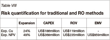
This 'double consideration' is shown in Figure 13 for the expected Cu production option, where the upside potential is represented by the horizontally traced area, and the hedging cost by the vertically traced area. Traditional valuation methods account only for the hedging side, punishing the project's value by overestimating risk.

 

 

Risk management application

In summary, a risk-based valuation methodology can be divided into four stages: planning for risk, assessing risk issues, developing risk handling strategies, and monitoring to see the change over time (Maybee, B., Lowen, S., and Dunn, P. 2010). Integrating RO into this process provides an effective risk-handling strategy for dilution. However, the main contribution of this study is providing the level of confidence for a given production rate, helping decisionmakers choose a strategy according to their risk aversion level and quantifying risk (Maybee, B., et al., 2009; McCarthy, 2002).

With this approach, it is possible to establish a clear relationship between the production rate and the probability of obtaining an expected project outcome. Figure 14 shows this relationship for the present case study: as production increases, the probability of achieving the expected targets increases and the life of mine decreases, until a technical limit is reached. This limit represents the maximum hedging level for this operation.

 

 

Conclusions and further studies

A real options analysis was successfully executed to measure the impact and manage the risk associated with dilution uncertainty in a mining project. The results show that risk quantification by real options yields values up to four times lower than traditional methods and provides transparent and reliable results. Furthermore, the real options method not only quantifies the hedging costs, but also takes into consideration the upside potential related to future management decisions, thus obtaining a globally optimized operation, rather than a local maximum result that is rarely achievable.

Even though this study focuses solely on the effects of dilution, a similar methodology may be applied to other mine planning variables such as ore grade, metallurgical recovery, and operational performance. These variables originate from three completely different areas of a mining project; however, the risk they all bring into the project is the same: the possibility of producing less metal than expected. This fact allows the handling strategies and monitoring processes to also be the same. In short, real options can very effectively be applied to manage risk associated with variables that affect the different processes downstream of the system.

Further studies should focus, on one hand, on creating risk clusters that share the same effect on the project's outcome (with their corresponding correlations). With this, it is possible to develop an integrated model that considers these clusters instead of single variables, and produce a global risk quantification model. On the other hand, further research could be done on the possibility of applying this methodology to short-term planning.

 

References

Akbari, A.D., Osanloo, M., and Shirazi, M.A. 2009. Reserve estimation of an open pit mine under price uncertainty by real option approach. Mining Science and Technology (China), vol. 19, no. 6. pp. 709-717.         [ Links ]

Amram, M. and Kulatilaka, N. 1999. Real options: managing strategic investment in an uncertain world. Harvard Business School Press. 246 pp.         [ Links ]

Botín, J., Guzmán, R., and Smith, M. 2011. A methodological model to assist the optimization and risk management of mining investment decisions. The Society for Mining, Metallurgy and Exploration Annual Meeting, vol. 11, no. 124. pp. 1-6.         [ Links ]

Botin, J., Del Castillo, F., and Guzman, R. 2011. Real options: a tool for managing technical risk in a mine plan. Proceedings of the 2011 Annual SME Meeting. The Society for Mining, Metallurgy and Exploration, Littleton, Colorado.         [ Links ]

Cardin, M.A., de Neufville, R., and Kasakidis, V. 2008. A process to improve expected value on mining operations. Mining Technology, vol. 117, no. 2. pp. 1-15.         [ Links ]

De Neufville, R. and Scholtes, S. 2011. Flexibility in Engineering Design. MIT Press, Cambridge, MA.289 pp.         [ Links ]

Diering, J.A. and Laubscher, D.H. 1988. Practical approach to the numerical stress analysis of mass mining operations. International Journal of Rock Mechanics and Mining Sciences & Geomechanics, vol. 25, no. 3. pp. 179-188.         [ Links ]

Dimitrakopoulos, R. and Sabour, S. 2007. Evaluating mine plans under uncertainty: Can the real options make a difference? Resources Policy, vol. 32, no. 3. pp. 116-125.         [ Links ]

Dimitrakopoulos, R., Martinez, L., and Ramazan, S. 2007. A maximum upside /minimum downside approach to the traditional optimization of open pit mine design. Journal of Mining Science, vol. 43, no. 1. pp. 73-82.         [ Links ]

Hudson, J.A. (ed.). 1993. Comprehensive Rock Engineering: Principles, Practice & Projects. Pergamon. 1st edn. pp. 547-583.         [ Links ]

Kasakidis, V.N. and Scoble, M. 2003. Planning for flexibility in underground mine production systems. Mining Engineering, vol. 55, no. 8. pp. 33-38.         [ Links ]

Martinez, L. and McKibben, J. 2010. Understanding real options in mine project valuation: a simple perspective. MININ 2010. Fourth International Conference on Mining Innovation, Santiago, Chile, 23-25 June 2010. Castro, R., Emery, X., and Kuyvenhoven, R. (eds). Gecamin, Santiago. pp. 223-234.         [ Links ]

Maybee, B. 2010. Risk quantification using quantitative tools. International Journal of Decision Science, Risk and Management, vol. 2, no. 1/2. pp. 98-111.         [ Links ]

Maybee, B., Dunn, P., Dessureault, S., and Robinson, D. 2009. Impact of development strategies on the value of underground mining projects. International Journal of Mining and Mineral Engineering, vol. 1, no. 3. pp.219-231.         [ Links ]

Maybee, B., Lowen, S., and Dunn, P. 2010. Risk-based decision making within strategic mine planning. International Journal of Mining and Mineral Engineering, vol. 2, no. 1. pp. 44-58.         [ Links ]

McCarthy, P. 2002. Feasibility studies and economic models for deep mines. Proceedings of ACG International Seminar on Deep and High Stress Mining, Perth. p.6.         [ Links ]

Mular, A.L. 2002. Major mineral processing equipment costs and preliminary capital cost estimations. Mineral Processing Plant Design, Practice and Control. Proceedings. Mular, A.L., Halbe, D.N., and Barratt, D.J. (eds.). Society for Mining, Metallurgy, and Exploration, Littleton, CO. vol. 2. pp. 310-325.         [ Links ]

Musingwini, C., Minnitt, R., and Woodhall, M. 2007. Technical operating flexibility in the analysis of mine layouts and schedules. Journal of the Southern African Institute of Mining and Metallurgy, vol. 107, no. 2. pp. 129-136.         [ Links ]

Ovalle, A.W. 2012. Mass caving maximum production capacity. MASSMIN 2012. 6th International Conference and Exhibition on Mass Mining, Sudbury, Canada, 10-14 June 2012. Canadian Institute of Mining, Metallurgy and Petroleum. Westmount, Quebec.         [ Links ]

Reichmann, W.J. 1962. Use and Abuse of Statistics. Oxford University Press. 352 pp.         [ Links ]

Rozman, L.I. 1998. Measuring and managing the risk in resources and reserves. Towards 2000 - Ore Reserves and Finance, Sydney, NSW, 15 June 1998. Australasian Institute of Mining and Metallurgy. pp. 43-55.         [ Links ]

Sabour, S. and Wood, G. 2009. Modeling financial risk in open pit mine projects: implications for strategic decision-making. Journal of the Southern African Institute of Mining and Metallurgy, vol. 109, no. 3. pp. 169-175.         [ Links ]

Samis, M., Martinez, L., Davis, G., and Whyte, J. 2011. Using dynamic DCF and real option methods for economic analysis in NI43-101 Technical Reports. VALMIN Seminar Series, Perth, October 2011. Australasian Institute of Mining and Metallurgy. pp. 1-23.         [ Links ]

Sayadi, A., Heidari, S., and Saydam, S. 2010. Study of key factors in geometrical and grade modelling of copper porphyry deposits. International Journal of Mining and Mineral Engineering, vol. 2, no. 1. pp. 59-77.         [ Links ]

Snowden, D., Glacken, I., and Noppe, M. 2002. Dealing With demands of technical variability and uncertainty along the mine value chain. Value Tracking Symposium, Brisbane, Queensland, 7-8 October 2002. Australasian Institute of Mining and Metallurgy, Melbourne.         [ Links ]

Torries, T. 1998. Evaluating mineral projects: applications and misconceptions. Society for Mining, Metallurgy and Exploration. Littleton, CO.         [ Links ]

Wang, T., and de Neufville, R. (undated). Identification of real options "in" projects. Systems Engineering: Shining Light on the Tough Issues. Proceedings of INCOSE 2006, Orlando, Florida, 9-13 July 2006. International Council on Systems Engineering, San Diego, CA.         [ Links ]

White, D.H. 1990. Geomechanics and Cost Effective Block Caving. Society for Mining, Metallurgy and Exploration, Littleton, CO.         [ Links ]

Whittle, G., Stange, W., and Hanson, N. 2007. Optimizing project value and robustness. Project Evaluation Conference, Melbourne, Victoria, 19-20 June 2007. Australasian Institute of Mining and Metallurgy. pp. 147-155.         [ Links ]

Williams Jr., R. 'Six Tenths Factor Aids In Approximating Costs'. Chemical Engineering, December 1947        [ Links ]

 

 

Paper received Aug. 2012
Revised paper received Apr. 2013

 

 

a This Software specializes in simulation and automation, developed by Systems Modeling, which uses SIMAN processor and simulation language.
© The Southern African Institute of Mining and Metallurgy, 2013. ISSN 2225-6253.