Pre-mining stress model for subsurface excavations in southern Africa

 

 

M.F. Handley

Principal, Hands on Mining cc

 

 

---

SYNOPSIS

This paper covers in situ stresses in the Earth's crust prior to any man-made disturbances, such as mining. It introduces the Southern African Stress Database, which contains primitive stress measurements obtained from locations spread all over southern Africa. The measured stress data shows large variability without any visible trends, except a relationship with increasing depth. The stress database is reviewed briefly, establishing means to measure the variability or dispersion in the measurements, and showing that the dispersion is not as much a result of experimental error as it is a feature of primitive stress. The paper demonstrates from the beginning that the state of stress in rock is highly variable, but that there are well-defined maximum and minimum limits to all the stress components in rock. Formal error analysis is introduced to check the consistency of the database and to separate out a database of consistent stress measurements for use in a primitive stress model. The aim is to provide a picture of primitive crustal stress based on objective stress measurements together with interpretations of how the primitive stress can be affected by the five main influences; namely, depth, rock mass properties, tectonism, isostacy, and erosion. Four elementary models for primitive stress are introduced and compared with the measured data. It is quite clear that none of the elementary models is sufficient to describe the data. In the absence of a better model, this paper suggests a generic model based on the Hoek-Brown failure criterion and the consistent stress database, since it incorporates the variability in the stress tensor that is likely to be encountered underground all over southern Africa. Rock engineers should take every opportunity to obtain local primitive stress data at every mining operation and civil engineering project, and to adjust the proposed model accordingly

Keywords: primitive stress, Southern African Stress Database, error analysis, generic primitive stress model.

---

 

 

Introduction

Rock conditions and the distribution of payable ore underground control the mining strategy adopted and the resulting mine layout. Mine stability then depends on the relationship between the strength of the rock mass and the total field stresses, which result from the mine layout. Since the field stresses are always the sum of the primitive stresses and the mining-induced stresses, both must be known to a reasonable degree of accuracy, since the risk of instability may need to be estimated both during mining and after mining has ceased. Either the primitive stresses must be obtained from in situ stress tensor measurements or from a good pre-mining stress model (initially limited to the depth of mining of 4 km), while the mining-induced stresses come from numerical models of the mine and the rock mass structure.

Rock stress data from in situ measurements is scarce because it is both difficult and expensive to obtain. Workable stress measurement technology became available to mining only during the 1960s (Leeman, 1965, 1968; Pallister, 1969). At the same time, means to calculate stress changes induced by mining were being introduced (Salamon, 1965; Salamon et al. 1965; Ortlepp and Nicoll, 1965). There are no good pre-mining stress models because of the difficulty and cost of obtaining stress data. This paper demonstrates that the pre-mining stress models currently used in rock mechanics are inadequate, and addresses the problem of deducing a generic primitive stress model for mining from the Southern African Stress Database.

The Southern African Stress Database is a good source of primitive stress data, compiled from stress measurements made all over southern Africa from May 1966 to October 1997 (Stacey and Wesseloo, 1998a). The compilers state that the database should be used for this purpose by the mining industry, but to date none of the data has appeared in the literature. There is another stress database known as the World Stress Map, which is built up from earthquake data worldwide (Heidbach et al., 2009). This database contains only eight records for South Africa, and none is suitable for building a primitive stress model for mining purposes.

The Southern African Stress Database

Stacey and Wesseloo (1998a) compiled the Southern African Stress Database under the auspices of the Safety in Mines Research Advisory Council (SIMRAC) to make all stress measurement data, previously contained in scattered tenders, contracts, internal reports, and other inaccessible documents, available to the mining industry. The measurements come from all over southern Africa, namely South Africa, Namibia, Angola, Mozambique, Malawi, Zambia, Zimbabwe, Botswana, Lesotho, and Tanzania. This stress database records only primitive stress measurements from mining and civil engineering projects; it does not include measurements of total mining stresses. The database contains 526 stress measurement records. Each record contains the date of the stress measurement, location, depth, stress components measured, and some information on type of measurement, rock formation, and rock type.

The records also contain the measured stress tensor components in the form of normal and shear stress components with reference to a coordinate system in which the positive x-axis is east, the positive y-axis in vertically upwards, and the positive z-axis is north (see Stacey and Wesseloo 1998a, 1998b for a complete description of the stress database). For the mining industry, it is preferable to use the South African Coordinate System, since most mines in South Africa use this system or a variant as a local coordinate system. The South African Coordinate System, also known as the Hartebeesthoek94 Coordinate System and implemented in South Africa on 1 January 1999, sets the positive x-direction as south, the positive y-direction as west, and the positive z-direction as vertically downwards (Wonnacott, 1999). Conversion of stress tensor components contained in the Southern African Stress Database to this system is trivial.

Where complete physical measurements of rock stress were undertaken, the stress tensor is reported in the form of principal stress magnitudes, their plunges, and plunge directions. In instances in which the stress tensor has been inferred indirectly from earthquakes or other indirect means, the data is incomplete in that either some or all the principal stress magnitudes or their directions, or some of both, are not reported. Of the 526 records in the database, 221 measurements were indirect and report the stress tensor partially. The reason for this is the nature of the measurement itself. For example, dog-earing in a borehole or scaling in an ore pass yields the maximum and minimum principal stress in a plane perpendicular to the axis of the excavation. The method cannot yield the magnitudes of the three principal stresses or their directions, therefore records using this method yield only part of the three-dimensional stress tensor. Other methods reported in the database that yield partial results include earthquakes, hydrofracturing, and other physical stress measurements that did not measure the full three-dimensional stress tensor. Stress measurements in which the total field stress (primitive stress summed with mining-induced stresses) are rare, and were not included in the stress database. The only ones known to the author are those by Leeman (1965), Deacon and Swan (1965), Gay (1979), and Handley (1987).

After excluding the 221 incomplete records, the remaining 305 records report the full stress tensor, all measured using physical methods, which will not be covered here but can be reviewed in Amadei and Stephansson (1997) or Ulusay and Hudson (2007, pp. 331-396). These records constitute the only data suitable for analysis and development of a crustal stress model applicable to mining. These records will be referred to in this paper as the Abridged Southern African Stress Database, or the abridged database. The abridged database of 305 records consists of 74 averages, 134 individual measurements that were included in the 74 averages, and 97 individual measurements that were not included in any averages. It therefore really consists of two separate databases: 134 + 97 = 231 individual measurements, and 74 averages computed from the 134 individual measurements. As a result, there is repetition in the abridged database because results from the 134 individual measurements are again reflected in the 74 averages. The small number of complete stress measurements emphasizes the difficulty and expense of obtaining complete stress data: in over 40 years, only 231 full stress tensors were measured over all of southern Africa, amounting to five or six measurements per year.

The most notable feature of the abridged database is the variability or dispersion of the vertical stress values measured (Figure 1). This was originally attributed to experimental error (see Gay 1975, pp. 448-449). Pallister (1969) estimates experimental error in his measurements to be 20%, yet he reports a stress measurement 2400 m below surface at East Rand Proprietary Mines Ltd, Boksburg, with a measured vertical component 43% below the expected vertical component for that depth. Stacey and Wesseloo (1998a) consider this measurement to be sound, grading it 'B' in their grading system with categories 'A' to 'E' going from 'reliable, i.e. at least 80% of the measurements in close agreement to 'results too variable, or irresolvable inconsistencies, and/or contradictory indications'. The classes of their subjective/quantitative system can be seen in Stacey and Wesseloo (1998b).

 

 

Figure 1 is a cumulative percentage frequency plot of absolute normalized error computed from the measured vertical stress and the expected overburden stress according to the formula after Taylor (1997):

where e is the percentage normalized error, σmv is the measured vertical stress component, and σ_ev is the expected vertical stress component due to the overburden weight. The cumulative percentages plotted in Figure 1 were then found by counting the number of measurements with less than 10% error computed using Equation [1], the number of measurements with less than 20% error, and so on up to 400% error, and then normalizing the results. This was repeated for each category 'A' to 'E'.

This plot was obtained from data in the Southern African Stress Database because there are 324 data available, which were classified into the five gradings by Stacey and Wesseloo (1998a, 1998b). There are 19 more records included in the plot than are contained in the abridged database (305 records) because these additional records do at least report a measured vertical stress component and an expected vertical stress component, even if the stress tensor reported is incomplete. The data includes 19 ungraded measurements that were lumped with those graded 'E', while the abridged database contains only eight ungraded measurements. No effort has been made to separate the averages from the other data in Figure 1 because it does not affect the overall pattern shown.

Figure 1 shows that the measured vertical stress component is widely dispersed around its expected value, even though it should be fairly well constrained by gravity and crustal equilibrium. The plot also shows that dispersion far exceeds the 20% experimental error cited above. Note that the subjective/quantitative method of grading the data (Stacey and Wesseloo, 1998b) does not reduce the dispersion in the higher grades with respect to that in the lower grades. For example, Groups A and C have almost equal dispersion below 20% error, and then Group C has lower dispersion than Group A above 20% error. The data is judged to be consistent, since Stacey and Wesseloo (1998a) concluded this after recalculating some results, and a second analysis below also shows that it is generally consistent. The dispersion in the data must therefore be a feature of the stress state in the Earth's crust.

Figure 2 shows a scatter plot of the measured vertical stress component versus the expected vertical stress due to the overburden weight obtained from the database. This diagram shows the dispersion in a different way, and does not show the classification of Stacey and Wesseloo (1998b). It highlights the example measurement of Pallister (1969), and shows that there are many other measurements with large differences from the expected result. There is no similar measure to display the dispersion of the horizontal stresses, which may be more widely dispersed than the vertical component, the only limits being compressive buckling, or tensile extension of the Earth's crust. This will be discussed in detail later.

 

 

Statement of problem and scope of paper

As has been demonstrated, there is a lot of dispersion in the primitive vertical stress component, even though it should be fairly well constrained by equilibrium requirements and gravity. The first explanation given above is the experimental error of 20%, but this is not enough to explain the observed dispersion of the vertical stress component (Figures 1 and 2). Either experimental errors are far larger than quoted, or there is a natural variability in the vertical stress component that comes about through the discontinuous structure of the rock mass. Stacey and Wesseloo (1998a, 1998b) do not discuss dispersion in the database.

The upper lithosphere is considered to be strong, crystalline, and brittle (Zoback et al., 1993) and therefore able to sustain large deviatoric stresses over geologic time, since creep rates are extremely low. Such large variability as seen in the stress database is therefore likely. To limit the scope, this study is confined to the upper lithosphere, where mining is now approaching 4 km below surface in relatively cool rocks that are subject to relatively low stresses, and where physical stress measurements have been made. It ignores the greater part of geophysical literature on lithos-pheric stress, which contains models to 30 km or more, and which takes account of creep in rock at both low and high temperatures.

Perhaps the most-cited and best-known treatise on rock stress forms the second chapter of Amadei and Stephansson (1997), who cover all the lithosphere stress models that had been published to that date. Many of these are not applicable to this study since they are regional, considering tectonic stresses in the oceanic and continental lithosphere. In describing a lithospheric stress model that could be applicable to mining, Rummel (1986) concluded that most laboratory tests of rock strength conformed to an equation of the form (σ₁-σ₃)_c = A+B (σ₃) ^1/2, where σ₃ is the effective confining stress, (σ₁-σ₃) is the peak differential strength of the rock, and A and B are constants dependent on the temperature of the rock. This formula is general in that it applies to the entire lithosphere, in rocks that are cool or hot, and in rocks deeply buried or near surface. Using it, Rummel (1986) was able to derive stress difference limits for reverse and normal faulting in both dry and wet conditions down to a depth of 30 km assuming a geothermal gradient of 25K/km. Although this work may be directly relevant to mining, it is considered to be the subject of long-term research, which will need far more extensive stress data than is available at present. Once this is in place, extension of the proposed pre-mining stress model to greater depths will be possible.

The first problem is to describe, and take account of in a consistent way, the dispersion of all the stress components in the Southern African Stress Database, not just that of the vertical stress component. This paper first describes semi-quantitatively how stress can vary in a discontinuous granular medium, and qualitatively how the primitive vertical stress can vary in a typical jointed and bedded rock mass. It goes on to establish whether the dispersion of the vertical stress component is natural or experimental in origin, by reviewing the consistency of the measurements in the abridged database. It then introduces a measure of dispersion, which can be used for all the normal stress components (vertical and horizontal alike), and also introduces limits to stress dispersion in the Earth's crust. It separates the consistent stress measurement data out of the database using error analysis and propagation of errors through calculations. Since this paper is addressed to the mining community, there is a brief introduction to the structure of the Earth's crust and upper mantle, which is included in a pre-mining stress model introduced later in the paper. This is followed by a review of the applicability of current pre-mining stress models by describing them and comparing them with stress measurements from a consistent database. Finally, it introduces a generic primitive stress model for a depth range covered by the stress measurements (<4 km), which can be used in the mining industry to determine the pre-mining stress state objectively.

This work concludes that the generic pre-mining stress model will need modification and refinement as more stress data becomes available. It also concludes that there is much to investigate, including a detailed re-evaluation of the Southern African Stress Database from the original strain relief measurements. A lot more research and data is necessary to produce a reliable primitive stress model for mining that could be extended to greater depths than those encountered today.

 

Assessment of stress in a discontinuous solid

A quantitative assessment of stress in a granular medium 5 mm on a side is shown in Figure 3 (after Handley, 1995).

 

 

Although the granular medium has been loaded vertically by uniform velocity boundaries at top and bottom, and free boundaries on the sides, intergranular movements and opening of cracks between grain boundaries have led to a non-uniform stress distribution in the medium. The larger stresses are now concentrated into 'grain columns' that are relatively stable, while more unstable columns have low stress. The thicker black lines in the picture are opening cracks between the grains.

The stresses are generally not parallel to the y-axis, despite loading of the medium being parallel to the y-axis. This picture is at a granular level and it shows that stress can be variable over very short distances, in this case, in fractions of a millimetre. The granular geometry model is not dissimilar to a jointed rock mass, which is undergoing uniform loading by deposition of sediment. By analogy, the vertical stress component could become variable by a similar mechanism of joint-bounded inter-block movements during loading.

On a larger scale of centimetres to metres, Figure 4 illustrates qualitatively how the vertical stress in a jointed and bedded rock mass may vary laterally. It is supported by successive strain relief measurements taken in boreholes by many authors (see for example Deacon and Swan, 1965; Leeman, 1965; and Handley, 1987). This diagram is intended to illustrate the effects of discontinuities on vertical rock stress. There are two major sets, namely the horizontal and the vertical discontinuities, the former being bedding surfaces and the latter joints. The visible and partly open discontinuities are shown as lines, and where the discontinuities are closed, they are not shown. Some of the discontinuities, both beds and joints, may also not be persistent, ending in solid rock. These will have the same effect as closed discontinuities from a stress point of view.

 

 

The axes provide vertical and horizontal scales of stress and distance respectively. The horizontal green line represents the expected average vertical stress magnitude for the appropriate depth in the rock mass illustrated. The green line also represents a line in the rock mass along which the vertical stress is known. This has never been done physically, that is why this is a qualitative illustration based on the quantitative granular model shown in Figure 3. The red line shows the actual qualitative distribution of the vertical stress in the rock. It shows that the rock may experience higher vertical stresses between the boundaries of two horizontal discontinuities, but lower vertical stresses immediately above or below the discontinuities, where they are open. This is because the stress has to be redistributed around the boundaries of the discontinuities. The concept is illustrated in Figure 4 by points 1-3 and points 4-6. Points 1 and 6 also show that the rock mass is able to support a vertical stress discontinuity across a vertical joint, much like the stress in a granular medium.

The red line represents the vertical stress magnitude at many points along a line for an elevation given by the green line. The profile of the red line (i.e. the position of local stress highs and lows) would change substantially if the vertical stress could be measured on similar horizontal lines a short distance above or below the green line. The vertical stress is therefore strongly influenced by local discontinuities in the rock mass. For equilibrium, the area between the green line and the horizontal axis must be equal to the area between the red line and the horizontal axis. Therefore a stress high at one point in the rock mass must be compensated for by a stress low at another point, with the two averaging out to preserve the observed equilibrium of the rock mass as a whole.

Thus on the very small scale of millimetres and the small scale ranging from centimetres to metres, brittle rock stress is seen to be variable. At large scales (tens of kilometres) it is also found to be variable, as demonstrated by Heidbach et al. (2009), Amadei and Stephansson (1997), and others. Since stress variability seems to exist at all scales, it can be extended to the familiar means of computing the vertical rock stress component for an imaginary vertical column of rock as shown in Figure 5. This shows that reaction forces (arrows representing the vertical force component on enlarged surfaces drawn to different lengths and in different colours to facilitate visualization) and therefore stresses at different points on the base of an imaginary rock column (this base could be a horizontal joint or bed) need not be equal. However, the formula for calculating the vertical stress, given by σ_ob = pgz (ρ = rock density, g = acceleration due to gravity, and z = depth below surface) actually computes an average vertical stress component for the imaginary surface at the given depth z. Overall, the point to remember is that the components of the stress tensor can be very variable in a natural rock mass, and that the normal means to compute them will yield averages.

 

 

Stress differences can be very significant over small distances in a rock mass, as has been demonstrated above on a granular scale over millimetres. Since typical strain gauges in a stressmeter are of the order of 10 mm long, this illustrates why adjacent stress measurements only 10 cm apart could be significantly different from each other (see Amadei and Stephansson, 1997 or Ulusay and Hudson, 2007 for descriptions of stressmeters). This also illustrates why several closely spaced stress measurements should be averaged to obtain a better picture of the overall stress state in a rock mass. Finally, it shows how stress measurements from several boreholes drilled in different positions may not be compatible with each other, and that this could be a source of inconsistency in some of the stress measurements in the Southern African Stress Database.

 

Assessing the quality of the stress measurements in the abridged database

In compiling the database, Stacey and Wesseloo (1998) reported that they found several results with errors, such as non-orthogonal principal stress directions. This led to their recalculating measurement results where they had access to the original strain relief data. This turned out to be an independent random check of the reported data, from which they concluded that all the reported data was correctly processed (Stacey and Wesseloo, 1998). Since the Southern African Stress Database does not provide any strain relief data, the author is forced to accept the finding of Stacey and Wesseloo (1998). However, their report suggests that not all results were checked, nor do they specify which results were recalculated, so more external checks have been performed by the author on all the data in the abridged database. This amounts to a complete re-check of the consistency of all the results in the abridged database using error analysis. This does not contradict or conflict with the work of Stacey and Wesseloo (1998); it merely re-evaluates the consistency of the database from another point of view.

 

Checking for orthogonality, normality, and agreement between the measured vertical stress and the expected vertical stress

The abridged database has been re-checked for the mutual orthogonality and normality of the principal stress direction vectors, and the agreement between the measured vertical stress component and the theoretical overburden stress determined from the measurement depth and rock mass density. These checks are reported in detail because they serve as useful information for future stress measurement checks, and because they are independent of the process used to arrive at the stress tensor results given in the abridged database.

Directional cosines of principal stress directions determine the orthogonality and normality of the principal stress vectors, as they are reported in the abridged database. Figure 6 illustrates how the directional cosines were determined. The normality of the directional cosine vectors is checked by finding the square root of the sum of the squares of the directional cosines for each principal direction. This result is by definition unity (see Appendix A for more detail on directional cosines). Departures from normality are reported in normalized percentage error form after Taylor (1997), using the equation:

 

 

 

where nc, and n ^def= 100 are the normality computed from directional cosines for the principal stress direction vector as projected onto a pre-defined coordinate system axis, and the defined normality of the direction vector respectively.

Dot products between the directional cosines of any two principal stress components in a principal stress tensor must be zero for the two components to be mutually orthogonal. The orthogonality error has to be computed in a different way, because the dot product is zero, which renders an equation like Equation [2] indeterminate. The deviation from orthogonality is therefore given in percentage deviation of the angle between two principal stress directions from π/2 radians, as follows:

The quantity o_c is the dot product between two vectors, in this case the principal stress directional cosines expressed as vectors, and it can take on a range of values given by -1 < o_c < 1, but for mutually perpendicular direction vectors, o_c = 0 by definition. The quantities given in Equations [2] and [3] are easily computed from the directional cosines on a spreadsheet.

The results appear plotted in Figure 7. The normality and orthogonality error frequency plots are both very similar because both are generated from the same set of directional cosines. Both appear in Figure 7, which shows that approximately 97% of the results (1340 measurements out of a total of 1386 - three normality and three orthogonality tests for each of 231 measurements) are less than 2% deviant from normality (n_c = 1.00) and orthogonality (equivalent to 1.8°). The averages are not included in the plot to avoid double counting.

 

 

The plot in Figure 7 does not adequately separate the consistent data from inconsistent data, but it does suggest a criterion of separation. The three normality and three orthogonality checks in each record amount to six possible criteria for excluding the record from further analysis, and if any one of the criteria is exceeded, then the record is rejected on the grounds that there may be an error in the calculations or measurements. On this basis, a total of 30 records are found to have absolute errors in normality and orthogonality exceeding 2%, amounting to 10% of the measurement records. This is larger than the 3% error suggested in Figure 7. The remaining 275 records consist of 66 averages and 209 individual measurements made up of 124 measurements included in the 66 averages, and 85 individual measurements, not included in any averages. Further checks in this reduced database showed that there was still inconsistent data. This indicated that more rigorous tests based on a more sophisticated error analysis were necessary to separate the consistent records from the inconsistent records.

Since the author did not have any information on the errors of measurement, an analysis based on inferred errors in the database became necessary. A good start is a check using an objective error criterion for the normality and orthogonality of the principal stress directional cosines. Since Figure 7 already displays that there is uncertainty in the reported azimuth and plunge angles for the principal stresses reported in the database, it is prudent to work with these and use their propagation through the calculations to check for inconsistency. The error analysis is carried out after Taylor (1997), the details of which are described in Appendix A.

The analysis described in Appendix A was repeated assuming three angular uncertainties, namely 0.5°, 1.0°, and 2.0°. The first angular uncertainty is based on the fact that nearly all the principal stress azimuths and plunges are reported to the nearest degree in the abridged database, which amounts to a maximum angular uncertainty of 0.5°. A total of fifteen criteria based on angular uncertainty were used to reject inconsistent records in the abridged database, namely the normality of the three coordinate axis vectors, the orthogonality of the three coordinate axis vectors, and the consistency of the nine stress tensor components. These can be reduced to twelve by the symmetry of the shear stresses. If a stress measurement record listed in the abridged database failed any one of the twelve inconsistency checks it was rejected. The results appear in Table I.

Table I shows that a progressive relaxation of angular uncertainty results in a larger number of records being accepted as consistent. There is no means to decide which angular uncertainty is preferable for the purposes of this paper. It appears from Figure 7 that by 2% error (1.8°), the frequencies have reached some sort of background value, so it seems that accepting an angular uncertainty criterion of 2° may be appropriate. This suggests that stress directions measured in rock are reported with a ±2° error, which is a judgment of the author and not a rigid criterion. It results in 75 records being rejected, amounting to 25% of the abridged database. All further analysis will be based on the remaining 230 records, which will be called the Consistent Database.

Errors between the measured vertical stress component and the expected overburden stress are given by Equation [4]. These errors are also easily computed by spreadsheet, and are shown in Figure 8. The plot shows a large spread of the vertical stress component about the expected vertical overburden stress, as has already been illustrated in the introduction. This plot also shows that averaging individual measurements tends to move stress data leftwards into lower error categories only in the higher dispersion categories (>20%). This is not expected, since averaging is a means of reducing dispersion. This plot again confirms that the vertical stress component shows strong dispersion around expected vertical stresses in the rock mass, for which Figures 3 and 4 provide an explanation. Since all the stress components and their directions are considered consistent, the variability must be a feature of the rock mass and not of experimental error.

 

 

Overall, one may conclude at this stage that the vertical stress state in the Earth's upper crust is extremely variable. It is also reasonable to assume from earlier discussion that the horizontal and shear stress components may have more degrees of freedom and therefore greater dispersion than is shown by the vertical component. This is explored next.

A general framework to describe dispersion and limits to dispersion of all rock stress components

A cross-section through Africa along the great circle 27.5° has been constructed to illustrate large crustal features. The section must be drawn on a great circle because the planes of great circles are perpendicular to the spherical surface. To simplify, this rather complex picture, the great circle can be considered to approximate the straight section line given by the small circle defined by latitude 27° South. The section of the Earth's crust, constructed by the author after Mooney et al. (1998), appears in Figure 9. This rather complicated description of the construction is necessary because the scale of the drawing is such that the sphericity of the Earth becomes significant. The section passes through Elizabeth Bay on the Namibian coast, more or less through the centre of the Witwatersrand Basin and the Vredefort impact feature, and finally through Kosi Bay on South Africa's east coast.

 

 

The main crustal features shown are the lithosphere, which consists of two layers, namely the green layer of rocks predominantly of sialic composition, and the light brown upper mantle, which consists of rocks of ferromagnesian composition. The term sialic comes from SiAl - the shortened term for rocks rich in silicon- and aluminium-containing minerals, which have a density of approximately 2500-2800 kg/m³, and the term ferromagnesian comes from FeMg, for iron- and magnesium-containing minerals with densities of about 3300 - 3500 kg/m³. The division between the lighter and heavier rocks in the lithosphere is known as the Mohorovičić Discontinuity, discovered by Andrija Mohorovičić in 1909, and in Figure 9 is defined by Mooney et al. (1998) as the base of the sialic crust. This discontinuity represents a seismic wave velocity high, which is approximately 5-10 km deep below oceanic crust, and 20-90 km deep below continental crust.

Mining has not yet penetrated the Earth's crust more than 4 km, which amounts to penetrating the top 4% of the lithosphere (0.06% of the Earth's radius), which is not even visible in Figure 9. The structure of the Earth with its thin, solid crust suggests that it is reasonable to assume that close to the surface principal crustal stresses should possess a vertical component due to gravity and two horizontal components that arise from predominantly horizontal forces in the crust (see Figure 9). The rationale behind this is that crustal stresses are driven primarily by gravity, which acts vertically, and then by geological processes such as burial, denudation, and horizontal tectonic forces in the crust induced by movements in the mantle, all of which are assumed to have effects on crustal stress vertically and/or horizontally. The fact that the measured results are generally not vertical or horizontal is probably only local, and the result of the anisotropy and geological history of the rock in which they were measured.

As stated above, the primitive stress tensor is gravity driven, therefore its principal components will tend to be vertical and horizontal, unless some relatively recent or current geological event has affected, or is affecting, the rock mass of interest. This has been confirmed approximately by measurement, with deviations having origins described above (see Amadei and Stephansson, 1997, pp. 30-31). Therefore shear stresses on vertical planes tend to be zero. The exceptions to this rule come from the completely different mechanism of plate tectonics, which can cause shear stresses on vertical surfaces at plate boundaries, for example the San Andreas Fault and its offshoots, and other similar geological environments where there is relative horizontal movement between plates (see Lowrie, 2007).

At mid-ocean ridges, where sea floor spreading takes place, vertical transform faults develop more or less perpendicular to the line of the mid-ocean ridge because some parts of the ridge generate new sea floor faster than others (see Lowrie, 2007). There is horizontal shear on these vertical faults. Horizontal shear can develop between two plates where one plate is being thrust below another, although this shear will tend to follow the plate down as it bends downwards into the mantle. In mountain building processes, all manner of phenomena come forward: thrusting and other similar mechanisms that would create horizontal shear stresses. The primitive stress tensor will therefore tend to have vertical and horizontal principal components, except where presently ongoing or recent geological processes have resulted in changes to this pattern. In brittle rocks such altered stress states may be preserved for a very long time.

In recognition of the above discussion, McGarr and Gay (1978) expressed the crustal stress tensor in terms of a vertical component and two principal horizontal components with directions named σ_v, σ_h1, and σh2 respectively (see also Amadei and Stephansson, 1997, pp. 30-31). These components are found from the measured principal stress tensor by converting its components to a standard coordinate system. If the database coordinate system is used, then the vertical normal stress component is σ_v = σyy, and the two horizontal principal stress components σ_h1 and σ_h2 and their directions with respect to north are found from σxx, σzz, and σxz, all of which lie in the horizontal plane. The stress measurement results are listed in this form in the Southern African Stress Database.

This representation is not a complete stress tensor, since only four of the six independent stress tensor components for three dimensions are given, i.e. shear stresses along any vertical planes are omitted, although they are included in the database. Note also that many geological structures such as faults, dykes, and joints are inclined with respect to the horizontal, so that shear has vertical components, but that these were probably induced by changes in horizontal and vertical forces only. They are ignored in this analysis, because there are no large active transform faults, sea floor spreading, or plate subduction taking place in southern Africa.

To simplify the variability of magnitude and direction of each stress tensor component, there is also a need to ignore the direction of the horizontal components in the analysis, because two tensor components acting in different directions are not directly comparable i.e. to treat the horizontal principal stress component values as scalars when dealing with them statistically. The directions of stress components will be reconsidered in the construction of the proposed pre-mining stress model later. It is now possible to introduce a simple measure of the variability or dispersion of any of the three normal stress components.

The scalar equivalent of stress in solids is pressure in fluids. Since fluids cannot sustain shear stress, pressure is the same in all directions. If rocks could not sustain shear stress, then the rock stress would always be equivalent to pressure, and this pressure would be the same in all directions surrounding any given point in the rock. It would vary linearly in proportion with its density and the depth as σ_lith = ρ_gz (ρ is the density of the rock, g is the acceleration due to gravity, and z is the depth below surface). In rocks, such a stress state is called a lithostatic stress state, and it can be used as a reference to obtain a measure of variability of stress in rock, because any deviation from the lithostatic state must involve the rigidity of the rock and one or more geological processes. Plotting the magnitude of the lithostatic stress versus depth as shown in Figure 10a results in a lithostatic line, which must be zero at surface, increasing with depth as shown.

 

 

The lithostatic stress can be considered to have a vertical component, and two horizontal components, all equal to each other, since the lithostatic stress state is the same in all directions. A measure of variability of any of the normal stress components σ_v, σ_h1, and σh2 is given by the scaled horizontal distance by which each of these components is removed from this line, as shown in Figure 10a. We can ignore the directions of the horizontal stresses, since there will always be horizontal lithostatic stress components parallel to the horizontal principal stresses. Thus it is possible to note only the deviation of the horizontal and vertical stresses from the lithostatic line, as shown in Figure 10a.

When dealing with more than one stress measurement, we can define dispersion in a manner similar to the definitions of variance and the standard deviation in statistics. The magnitude of the lithostatic stress is linearly related to depth as described above, and this substitutes for the mean used in statistics to calculate the variance, since it is the average stress for that depth (see Figure 4). The lithostatic stress is therefore the expected stress at the depth of the measurement - this is equivalent to the mean in statistics. The average deviation from the mean for all the stress components is given by:

where â_sigv is the average deviation for the vertical stress component, σv(i) are the vertical stress measurements, σlith(i) are the corresponding lithostatic stress values for the respective vertical measurements at their respective depths, and N is the number of data used in the calculation.

Depth is automatically eliminated in Equation [4], because the expected value of the lithostatic stress (the mean) is depth dependent, and so is the measured stress depth dependent. To find â_sigh1i and â_sigh2 the values for the maximum horizontal stress σh₁ and the minimum horizontal stress σh2 are substituted for the vertical stress component in Equation [4] to find the average variance and deviation for these components, but the corresponding lithostatic stress data remain the same.

Using the lithostatic stress as the equivalent of the mean in Equation [4] is correct, since subtracting the horizontal stress data from the lithostatic stress data at the equivalent depth is physically meaningful, because there is always a lithostatic stress direction parallel to the direction of each measured horizontal stress component. We have to ignore the directions of the differences when summing up the squares of the differences and dividing by the number of data in the sum. The name average variance is given for the average of the squared differences, while the square root of this quantity is called the average deviation. These name changes differentiate them from the standard statistical definitions of the variance and standard deviation.

Neither the average variance nor the average deviation can have a direction ascribed to them. A total of twelve average deviation estimates can be found for the abridged database, where the measurement records are split into the averages and the individual measurements, and the consistent database split in the same way, as shown in Table II.

The most important feature common to these two databases is that the average deviation of the horizontal stresses from the lithostatic line is not affected by averaging stress measurements to reduce dispersion, or by selecting the consistent database from the abridged database. This suggests that the stress state in rock is intrinsically variable, and must be accepted as a very important feature of crustal stresses. In fact, the stress state seems to be so variable that including inconsistent data from the abridged database does not materially affect the average deviation. The averaged measurements also have higher average deviations than do the individual measurements, which suggests that averaging individual stress measurements has not reduced the dispersion. This is also partially confirmed by Figure 8.

In addition to this measure of dispersion, there are definite limits to the range of possible stress states in the Earth's crust governed by the strength of the rock. If one assumes that the southern African subcontinental rock mass will fail at stresses predicted by the empirical Hoek-Brown failure criterion, then one can conjecture the stress limits at which processes such as jointing, faulting, intrusions, and mountain-building may take place. The Hoek-Brown failure criterion, introduced by Hoek and Brown (1980), is given by:

where σ₁ and σ₃ are the maximum and minimum principal stresses respectively, σc is the uniaxial compressive strength of the rock, m is a Hoek-Brown parameter that depends on the rock type, and s is a second Hoek-Brown parameter that depends on the degree to which the rock is dissected by discontinuities. Although Rummel (1986) may have proposed a more general limit to crustal stresses, the author chooses the Hoek-Brown failure criterion for this purpose because it is well known in the mining industry, it is based on a large experimental database, and it is applicable to relatively cool and shallow rocks where mining is currently taking place.

In order to determine the minimum possible horizontal crustal stress, first assume that the maximum crustal stress is vertical and equal to the overburden weight i.e. σ₁ = ρgz, and solve for the minimum possible horizontal principal stress σ₃ that can exist in the Earth's crust by manipulating Equation [5] into the general solution for a quadratic equation in σ₃:

Choose the negative root because this gives a meaningful result for the minimum possible σ₃ given that σ₁ is vertical and equal to the overburden weight. Equation [6] renames σ3₁ as σhmin, in order to avoid confusion with the standard principal stress names used in the Hoek-Brown failure criterion and elsewhere, and to denote that this is a minimum crustal stress limit or tensile limit. The measured minimum horizontal principal stress data (σh2) listed in the abridged database must always be greater than or equal to the minimum crustal stress for stability.

To find the maximum possible horizontal stress that can exist in the Earth's crust, one must assume that the minor principal stress is vertical and equal to the overburden weight, that is σ₃ = ρgz. The maximum possible stress is now horizontal and given by σ₁, which is obtained directly from the Hoek-Brown equation for all depths z:

The positive root must be selected for a meaningful answer, and the resulting maximum possible horizontal crustal stress σ₁ is renamed σ_hmax in the model. This will avoid confusion with the standard principal stress names used in the Hoek-Brown failure criterion and elsewhere denoting that this is a maximum crustal stress limit or compressive limit. The measured maximum horizontal principal stress data (σ_h1) listed in the abridged database must always be less than or equal to the maximum crustal stress limit for stability.

Figure 10b, c, and d show three general cases of an overall crustal stress state. In the first case (Figure 10b) the crust is in relative tension. Here, the horizontal stresses are both less than the vertical stress, a condition that is commonly seen in the deep gold mines in South Africa (see measurements in Figure 11 below 2000 m). As can be seen from the diagram the crust is still in horizontal compression except near to the surface. The tensile limit is the minimum possible stress in the crust if the maximum stress is equal to the overburden weight. The difference between σ₁and σ₃at all depths is governed by Equation [5], while the tensile limit is computed using Equation [6].

 

 

Direction can be accounted for on a surface map on the right of the plot in Figure 10b, which shows a larger relative tension in a NW-SE direction, and a smaller relative tension at 90° to this in a NE-SW direction (these directions will be determined by the stress measurement data but are arbitrary in the diagram). At depth, these relative tensions will be compressive, but they could be tensile near surface, as suggested by the tensile limit in Figure 10b. Such a crustal condition would arise if the surface were undergoing uplift through upwelling mantle rock below the continental crust, or surface rock being eroded and deposited elsewhere. The geological structures that result are the intrusion of dykes and sills, and the development of normal faults and joints.

Figure 10c shows the crust in relative shear, in which one horizontal stress is less than the overburden weight and is at the lowest possible stress limit given that the other horizontal stress limit is greater than the overburden weight. The difference between σ₁ and σ₃ is governed by Equation [5]. There are many measured stress states in this category scattered across the full range of depths above 2000 m in Figure 11. The maximum shear stress in the crust is then half the difference between the two horizontal stresses, and would result in N-S and E-W faults with vertical dips and horizontal relative displacements, assuming the directions for the horizontal stresses as shown in the diagram. The author emphasizes again that the direction of the faulting is a result of the arbitrary choice of direction of the relative tension and compression in the Earth's crust, chosen for illustration of the concept in Figure 10. The intermediate stress in this case is the overburden stress.

Figure 10d shows the crust in relative compression where the smallest principal stress is vertical and equal to the overburden weight and both horizontal stresses are larger than the vertical stress. The compressive limit is the maximum possible stress that can exist in the crust if the minimum stress is vertical and the result of the overburden weight. At the compressive limit, folding (mountain building), thrust faulting and reverse faulting may develop. The difference between σ₁ and σ₃ is again governed by Equation [5], and the compressive limit is calculated using this equation while assuming that σ₃ is the minimum principal stress and is derived from the overburden weight. Given the direction of maximum compression on the accompanying map, folded mountains would form in a NE-SW trend, while reverse faulting and thrust faults would form in N-S and E-W conjugate pairs (these directions again obtained from the arbitrary choice of relative compression directions). Many of the stress measurements above 500 m exhibit a state of relative compression.

The patterns of stress distribution given by the stress measurements are not easy to interpret, and much more stress data is necessary to gain a better understanding of stress in the Earth's crust. The next step in this paper is to compare the stress measurement data with four simple mining stress models that have been used as a means to estimate the pre-mining stress state.

 

Four simple pre-mining stress models

The primitive stress tensor is the result of the geological history of the rock mass. The major factors influencing the primitive stress tensor are depth of burial, the rheological properties of the rock mass, tectonism, isostacy, and denudation. Secondary factors include topography, heating and cooling, groundwater, and weathering. Descriptions of the effects of these factors are given by Jaeger et al. (2007), Brady and Brown (2006), Ryder and Jager (2002), Amadei and Stephansson (1997), Hoek and Brown (1980), Jaeger and Cook (1979), McGarr and Gay (1978), and Gay (1975) amongst others, and will not be covered here. The measurement data in the plots all comes from the consistent database, and is included in four simple models of pre-mining stress. This data, together with the simple models, highlights how simplistic the pre-mining stress models are, and how poorly the crustal stress tensor is known.

Lithostatic stress model: Heim's Rule

This model assumes that all rock masses, regardless of how brittle they are, will creep under deviatoric stress conditions in geologic time. If the rock mass remains geologically undisturbed for sufficiently long, the deviatoric stress state will eventually become lithostatic, which is easily predictable with the simplest of models. This model assumes that the stress state in the rock mass is everywhere lithostatic; that is, the vertical stress component is a principal stress, and is equal to the stress due to the overburden weight, while the horizontal stress is the same in all directions, and equal to the vertical stress. This means that every direction in the rock mass is a principal direction, and that there can be no shear stress anywhere. The model is expressed as follows:

assuming a convenient coordinate system such as the South African Coordinate System, commonly used on the mines (Wonnacott, 1999). Note that by default, the conjugate shear stress pairs should always be equal for rotational equilibrium i.e. τ_xy = τ_yx: τ_xz = τ_zx : τ_yz = τ_zy. Because the three normal stresses are principal stresses, Equation [8] can be re-expressed as follows:

in which every direction is a principal direction because the rock mass is completely free of shear stress.

Present or past geological processes will result in a deviation from this pattern in the rock mass. Therefore, any deviation from this stress state in any rock mass is indicative of previous stress states from previous geological processes being preserved, or currently developing as a result of current processes. Even a process as seemingly insignificant as erosion can have a very significant effect on the stress state, as will be demonstrated later.

The lithostatic stress state, or a stress state approximating it, does exist in some rock masses and soft plastic materials, for example salt, peat, saturated clay, or potash. This stress state develops because the material will creep under deviatoric stress and establish lithostatic conditions in a short (geologically) time, perhaps ranging from years to millennia. The rate of creep will depend on the magnitude of the stress components and the material properties. A plot of the measured stress results versus the expected stress tensor components for a lithostatic stress state appears in Figure 11. This plot suggests that the rock mass stress state is generally not lithostatic. Because the measured data is so sparse, this conclusion cannot be assumed to be true everywhere in South Africa.

Three measurements in the consistent database approximate the lithostatic stress state, namely those at Beatrix Mine, Impala Platinum, and the Inanda Wiggens Tunnel (see Table III). The other two come from the abridged database, but are considered to be inconsistent. This does not mean that the lithostatic stress state does not exist in South Africa - the measurement data is simply too sparse to draw such a conclusion.

Rigid confinement model

The rigid confinement model assumes that rock is elastic, and that its Poisson's Ratio dominates the stress state to which it is subjected. This stress state develops in sediments, which during burial and the consequent vertical loading, are prevented from expanding laterally by the surrounding sediments. The Poisson's Ratio v of the unconsolidated sediment is assumed to be the same as that measured in the sedimentary rock millions of years later. This is highly unlikely to be true, but if so the Poisson effect, easily derived from the equations of elasticity, gives rise to equal horizontal stresses related to the vertical stress by:

assuming a system of axes referenced in the equation, with conjugate shear stress pairs being equal for rotational equilibrium. Again, because the normal stress directions are principal directions, the above equation can be re-expressed as follows:

where σ₁ is vertical while σ₂ and σ₃ are horizontal.

Figure 12 contains a plot of the stress data together with the expected stress components with depth according to the rigid confinement model, assuming v = 0.25. As is evident from the plot, the stress data displays far too much spread to give any indication that there are any instances in which this model may be true. Then, the measured horizontal stresses are never equal, as is predicted by Equations [10] and [11]. This could arise from anisotropy, but the overall loading directions of recent and earlier tectonic events are more likely to have resulted in the differences in measured horizontal stresses.

 

 

Furthermore, the rigid confinement from the Poisson effect will be magnified during burial, since any horizontal linear dimension must decrease linearly with increasing depth until it becomes zero at the Earth's centre. Therefore the rock will experience isotropic horizontal compression as a result of burial, which will result in larger horizontal stresses than predicted by Equations [10] and [11]. This model is unlikely to produce a good picture of stress in any rock mass anywhere, regardless of the value of the Poisson's Ratio. The next model addresses the effects of burial and uplift on the horizontal stresses.

Erosional/burial model

The erosional/burial model, after Price (1966), Voight (1966), Gay (1975), and Haxby and Turcotte (1976), and others, assumes that the crustal stress consists of a vertical component due to the overburden and two horizontal components that may be equal or unequal. The three components are principal stresses, and they vary linearly with depth. In this model the rock mass is subject to a stress state at depth that is subsequently relaxed both horizontally and vertically by the erosive removal of overlying strata, which results in its isostatic uplift or isostatic rebound. The opposite happens when an existing rock mass has sediments deposited on it. It experiences an increase in vertical stress due to the accumulating overburden, and an increasing horizontal stress due to subsidence as more material is deposited. In what follows, we will concentrate on erosion or denudation and rebound, although the equations to describe the phenomena are equally applicable to burial and subsidence. Only the boundary conditions at the commencement of one or the other process may be different (for example surface stresses at the time of commencement of burial, or crustal stress at the time of commencement of erosion).

The vertical stress relaxation rate is assumed to be directly proportional to the thickness and density of the overlying strata removed, and is therefore linearly related to the thickness of overburden removal. The horizontal stress relaxation rate is also linear. The same would apply to burial; here the density of the deposited sediments is possibly lower than the density of the consolidated overburden in the erosional case. Even with these differences, the equations remain the same, and therefore the discussion will continue assuming denudation and uplift.

The horizontal elongation of rock rebounding isostatically equates to a normal horizontal strain rate of 1.6 x 10^-4/km uplift, assuming Earth's radius to be approximately 6367 km. There is also the linear relaxation of vertical stress with overburden removal, which results in a linear relaxation of the horizontal stress through the equations of elasticity.

The horizontal stress need not be zero at surface, whereas the vertical stress must be zero. Haxby and Turcotte (1976) incorporate thermally induced expansion and contraction of the rock mass depending on the geothermal gradient and its depth of burial. They assume that rocks remain elastic at temperatures below 300°C, while above this temperature they flow plastically, removing deviatoric stresses and causing the stress tensor to approach the lithostatic state (Heim's Rule). This is an important paper, although the author does not agree with their assertion that the removal of overburden pressure has a compressive effect on the rock mass. The full derivation of the effects of erosion and isostatic uplift appears in Handley (2012), since it differs slightly from that of Haxby and Turcotte (1976). The equation for horizontal stress changes due to subsidence or uplift and thermomechanical effects derived in Handley (2012) is given by:

These effects are all linear, which will later be shown to be an important feature of stresses near the surface (above 10 km deep). Table IV contains the mechanical and thermal effects due to erosion of -1 km of continental crust using Equation [12] and the equation derived by Haxby and Turcotte (1976) for comparison.

Equation [12] predicts that the horizontal stress rate with erosion is slightly more than the vertical stress rate in the case of sandstone, while for limestone, granite, gabbro, quartzite, and marble the horizontal stress rate is less than the vertical stress rate. The Haxby and Turcotte (1976) analysis results in far greater horizontal stress rates than does Equation [12]. The latter is probably more plausible because the Haxby and Turcotte (1976) equation predicts strongly compressive stress states at surface, unless the horizontal stress at depth is always considerably less than the vertical stress (see Figure 13).

 

 

If there are lithostatic stresses at depth, the Haxby and Turcotte (1976) result precludes the development of vertical jointing in rock (see Price, 1966 and Figure 13) - a phenomenon that is seen everywhere. Haxby and Turcotte (1976) themselves assert that rock stress is probably lithostatic at temperatures above 300K, equivalent to a depth of 11 km if a geothermal gradient of 25 K/km is assumed. Although this is probably not true (earthquakes can originate at depths much greater than this), for the purposes of this paper it is assumed true in stable continental conditions such as those in southern Africa, and is therefore the basis of the plot in Figure 13. The best-fit lines described in Figure 13 are explained by Tables V and VI, Equation [13], and Figure 14.

 

 

Equation [12] predicts that the horizontal stress rates are fairly close to the vertical stress rates, allowing the horizontal stress to be either mildly tensile or mildly compressive at surface, depending on the state of stress before erosion and uplift takes place, and also on the rock properties. This allows for the formation of vertical joints as well as the observation that there are often compressive horizontal stresses at surface, if the rock mass is in a more or less lithostatic stress state before erosion. Both phenomena are nearly always present at surface, suggesting that the rock mass is most often in a lithostatic stress state or close to it when deeply buried. According to the geothermal gradient, rocks reach temperatures of 300°C between 11 and 12 km below surface, so from this depth downwards the stress state should be lithostatic or near to lithostatic. Rocks from this depth exposed at surface would then be marginally in horizontal tension or compression if Equation [12] is correct, which is the case observed all over the world.

It is well known that the continental rock mass near surface is seldom in a lithostatic state of stress (at least above 3000 m, as confirmed by the measurements in the consistent database), which suggests that the erosional model is important and significant, but it is not the only mechanism at work in determining crustal stresses near surface. The model appears to be too simplistic, possibly for the following reasons:

1. The rigid horizontal confinement at the continental boundaries is almost certainly not true (Haxby and Turcotte, 1976 also mention this fact)
2. Uniform erosion over an entire continent with removal of the eroded material from the continent is an oversimplification of typical erosional and deposition patterns observed globally
3. Uniform rock density is not the case in a homogeneous continental rock mass
4. The geothermal gradient is not uniform, since it varies locally and regionally
5. Assuming a homogeneous, amorphous continental rock mass is incorrect, because it contains geological structure such as joints, faults, dykes, sills, dipping and folded strata, rocks of different texture and type, and many other structures that could have a significant effect on the stress rates induced by erosion, subsidence, and temperature
6. Besides denudation and deposition of denuded material, mantle plumes, sea floor spreading, vulcanism, and subduction of oceanic crust at plate boundaries provide additional mechanisms that influence the stress state in continental crust 7. Detailed crustal stress data may not support the overall linearity of the model, which is supported by the currently available data (see below).

The linear denudation/depositional model described above is further tested near surface by fitting least-squares best-fit lines to the measured data for the vertical and two horizontal stress components versus depth. The correlation coefficients for the stress components versus depth for different collections of measurements appear in Table V.

The correlations are very good, even though the data comes from different locations across southern Africa, from rock masses with differing geological histories, but all in a similar stage of uplift through erosion and mantle upwelling (McCarthy and Rubidge, 2005). They suggest that about 80% of the variance in the stress data is explained by the depth. The 'A'- and 'B'-graded data selected by Stacey and Wesseloo (1998) show significantly improved correlation coefficients. Because of the good correlations one should conclude that there is a linear relationship between the measured stress components and depth, and that the thermomechanical model presented above may have some merit near surface if some adjustments are made to the boundary conditions. It is unlikely to be correct for the whole section through continental crust, and this should be the subject of further geophysical research in the long-term.

A near-surface pre-mining stress model showing a linear relationship with depth can be constructed from Table VI and the ideas of Price (1966), Voight (1966), Gay (1975), and Haxby and Turcotte (1976). The author first chooses a depth of 3000 m at which to define the best-fit stress state because conditions will not be significantly different from the depth of the deepest measurement in the database at 2778 m below surface. The stress state at 3000 m is determined for each horizontal stress using the intercepts and slopes of the leastsquares best-fit lines for the individual measurements from the consistent database in Table VI.

The same is done for the vertical stress component, this time using the slope and intercept for the least-squares best-fit line determined for the overburden stress determined from each measurement site. Again, the individual measurements from the consistent database were used. The reason for this choice is that the slopes determined for all the other datasets in Table VI are probably to too low for known densities of common crustal rocks (see vertical stress rates for different rock types in Table IV), with the exception of the 'A'- and 'B'-rated data from Stacey and Wesseloo (1998), where the slope is possibly too high. This point should be investigated in future research. A negative term (h - 3000) multiplied by the stress gradient with depth is added, so that a linear plot of the stress component versus depth is obtained. The slopes and intercepts are rounded so that the equations provide results to the nearest megapascal. The resulting equations are:

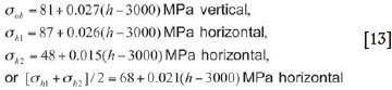
The consistent database stress measurements together with the straight lines from Equation [13] appear plotted together in Figure 14. The naming of the principal stresses in Equation [13] separates the vertical component from the two horizontal components because Figure 14 shows that both a_h1 and a_h2 are greater than a_ob near the surface, and both are less than a_ob at depth. This makes the normal naming convention of principal stresses impossible to apply.

Like the other models already described, the denudation model fails to provide a good visual fit to the data. The directions of the horizontal stresses cannot be specified in Figure 14, but local conditions on a mine will often indicate their directions unambiguously. There is still much work to be done in this area before any conclusions about the validity of one result or the other can be made. For the present, the scarcity and variability of the data and its being sourced from different geological environments may obscure the true patterns. These factors will be considered when building a generic pre-mining stress model.

Mine model

This model is derived from the deep-level gold mines of South Africa, where early stress measurements provided guidance for the assumption that the maximum principal stress was vertical, with the two horizontal principal stresses usually assumed equal and to be about half the vertical stress, i.e. a constant fraction of the vertical stress. This constant of proportionality became known as the k-ratio, which is defined as:

Subsequent stress measurements suggested that the horizontal stresses ranged between 0.4 and 0.8 times the vertical stress, which is shown in Figure 15. The equations for the simple tabular model are given by:

 

 

 

The platinum mines in South Africa also use this model, but in some cases assume the horizontal stresses to be equal to or greater than the vertical stress component.

From the few measurement data available from the gold mines, it appears that the stress tensor has a major principal component perpendicular to the bedding, the intermediate principal component is horizontal, parallel to the strike of the strata, and the minor principal component is parallel to the dip and dip direction of the strata. This pattern is faintly visible in the Carletonville Goldfield, and accounts for the observations that strike-stabilizing pillars are unstable - they punch into the footwall in the back areas - while dip-stabilizing pillars are stable, hence the success of sequential grid mining with dip pillars (Handley et al. 2000).

The vertical component of stress (parallel to the gravity vector) must be equal to the overburden weight, so this puts a limit on the size of two tilted components of the principal stress tensor, namely the component perpendicular to the strata, and the component parallel to strata dip. There are variations to this, especially near faults and dykes, which have been confirmed by observed changes in mining-induced seismicity near faults and dykes. It is therefore possible that non-zero shear stresses develop on vertical surfaces such as dyke boundaries and faults. There is virtually no physical information on this except for papers on stress measurements near dykes (Leeman, 1965; Deacon and Swan, 1965; and Gay, 1979).

Figure 16 contains the plot of measured k-ratios versus depth, inferred k-ratios obtained from the denudation model, and maximum and minimum possible k-ratios from the Hoek-Brown Failure Criterion (see Figure 17 for minimum Hoek-Brown parameters of crustal strength derived from the measured stress data). It is apparent that the measured k-ratio is definitely not constant with depth, and that there is a large spread in values. The superimposed denudation k-ratio curves on the data in Figure 17 produce a qualitatively better fit to the data than any of the other models, even though the linear stress curves produced by the denudation model in Figure 14 do not fit the data any better than any of the other stress models shown.

 

 

 

 

 

Voight's (1966) denudation model k-ratio fits the k-ratio obtained from the least-squares best-fit curve of the maximum measured horizontal stress data and the leastsquares best-fit curve of the measured vertical stress data (see Equation [13] for the parameters of these curves). The Hoek-Brown-derived limits of the k-ratio provide maximum and minimum limits to the k-ratio data for all depths after the concepts introduced earlier in Figure 10, and the derivation of the limit parameters discussed below.

 

Proposed pre-mining stress model

A good pre-mining stress model should recognize two facts: 1) that all stress states from the lithostatic state to a state of tensile or compressive crustal yield exist in every rock mass, and 2) the denudation model discussed above and encapsulated in Equation [13] and Figures 13 and 14 must provide a reasonable approximation of near-surface stress states. These assertions are supported by geological structure everywhere, which suggests that crustal rocks have been subject to successive stress states ranging from the tensile yield limit to the compressive yield limit several times in the geological past.

The tensile yield limit is manifested by joints, igneous intrusions, and normal faults, which could have developed in many different directions as a result of several separate episodes over geological time. Likewise, the compressive limit is imprinted on the rock mass in the form of reverse faults, folding, and mountain building. In addition to these extreme states, the rock would have been subject to every stress state in between. All rock masses in southern Africa exhibit geological structure consistent with both crustal stress extremes, in that both the tensile and compressive features are nearly always present.

The observed variability of stresses in the crust is so high that the probability of measuring a stress state close to the crustal strength, either in tension or compression, must be reasonably good. In addition, there can be considerable variation in the vertical stress due to rock mass structure. If the consistent database contains measurements of crustal stress states close to compressive and tensile failure, then fitting yield curves to the outermost measurements may provide a good indication of actual limits to crustal stress. This has been done in Figure 17, with the parameters given in Table VII.

 

 

These parameters were found by fitting Hoek-Brown yield curves to the outlying stress measurements. The Hoek-Brown limit curves predict a horizontal stress range between -11 MPa and 30 MPa at surface, obtained by setting σ_c = 60 MPa on average, and setting the s-value arbitrarily at 0.25, to represent widely-spaced joints in an essentially granitic continental rock mass. The vertical overburden stress is assumed to be σob = 0.027z, since this is the best-fit line slope for the overburden stress estimated for 180 individual measurements in the consistent database.

By definition, the m- and s-values must be the same for both sets of curves because they describe one continental rock mass composed of many different rock formations. Assuming the s-values are the same, and placing the curves such that they pass though the centre of gravity of the extreme values, we can find m-values by the solution of the equations. The results appear in Table VII. The m-values found for σ_hmin and σ_hmax differ only by 7.5%, which should be zero for the same rock mass, as stated above. They also provide good estimates of the k-ratio limits, shown in Figure 16.

These results are thus accepted for the crustal rock mass and used to plot the stress limits in Figure 17. The consistent database stress measurements appear in the plot to provide a visual indication of the stress limit curve fits to the data. The fact that the m-values for an assumed fixed s-value are similar but not the same can be considered to be the result of natural variability in the rock mass. since the extreme measurements in the consistent database were not made in the same location. In addition, the database used seems to provide a relatively good picture of the crustal stress extremes, and supports the supposition that the data-set contains stress measurements close to the crustal stress limits.

The fits of limit curves to the stress data have not contributed much more towards a pre-mining stress model. However, partitioning the space between the lithostatic stress line and the stress limit curves and determining the probability that a stress state will be found in any of the partitions will contribute much more toward a generic pre-mining stress model for southern Africa. Figure 17 shows the divisions, with the 180 stress data measurements from the individual measurements from the consistent database superimposed. The probabilities were determined from counts of the number of measurements of σ_ob, σ_hmin and σ_hmax that lie in each division, and dividing these by the total number of measurements performed. The counts were done on the 180 individual measurements from the consistent database, since including the 50 averages would have resulted in double counting. This procedure was repeated for the depth ranges 0-300 m, 300-1000 m, and 1000-3000 m, and plotted as the probability curves in Figures 18-20. The probabilities determined from these curves are summarized in Table VIII.

 

 

 

 

 

 

Figure 18 shows that the pre-mining stress above 300 m tends to be lithostatic, although there is variation in all three of the components on both sides of the lithostatic line. The maximum horizontal stress tends to be bigger than the vertical overburden stress between 0 and 300 m below surface. The minimum horizontal principal stress is generally equal to the vertical stress between surface and 300 m. From 300 m to 1000 m there is still a peak around the lithostatic stress line for the vertical stress component, while the two horizontal stress components are now more spread out, with the maximum horizontal stress being larger than the overburden stress, and the minimum horizontal stress being smaller than the overburden stress. Between 1000 m and 3000 m there are only 19 consistent stress measurements, which are insufficient to provide any definite trends. It appears that the vertical and maximum horizontal components are equal, and that they peak weakly on the lithostatic line. The minimum horizontal stress tends to be lower than the other two components. Much more data will be necessary to clarify these trends.

The most common stress state in the lithosphere is likely to be lithostatic, with increasing deviations from this state at shallower depths, decreasing to the purely lithostatic stress state once molten rocks are reached in the mantle. The depth range of the stress measurements in Figures 18 to 20 is too small to show this trend, but they do show a tendency toward the lithostatic state. Certainly, igneous rocks are liquid when they are emplaced, hence their stress states will always start in the lithostatic state. Cooling and other effects will alter this stress state later.

The same can be said for sedimentary rocks: the pore-water and sediment mixture will almost certainly behave as if it were a liquid prior to solidification, resulting in a more-or-less lithostatic stress state at the time of formation - in direct contradiction of the rigid confinement model discussed above and found not to be in agreement with the stress measurements. The initial stress state at solidification (lithifi-cation) is likely to be lithostatic until it is altered by other geological processes after formation. Metamorphic rocks may also start in the lithostatic stress state if they have undergone partial melting. Sometimes the fabric of metamorphic rocks (for example the alignment of platy minerals such as mica) show that the rock was subjected to anisotropic pressure, and that the rock was probably able to sustain the deviatoric stress at the time. Such rocks probably were not in the lithostatic stress state once they had cooled.

The way to use the probabilities in Table VIII is to first select the depth range in which the mine or part of the mine falls (for mines deeper than 3000 m, use the 1000-3000 m range). For example, Table VIII suggests that a mine in the 0-300 m range will find that the minimum horizontal stress is equal to the overburden stress about 36% of the time, exceeding it 30% of the time, and is significantly less than the overburden stress about 34% of the time.

This means that, since stress variations appear to exist in rock at all scales, variations such as these will be seen both on small and large scales. This will be manifested in the haulage by zones centimetres to metres, and even tens of metres long, where ground conditions are bad and the tunnel needs extra support. This will happen only where the stresses are extreme enough to cause rock instability near the tunnel periphery. These poor areas could be interspersed by good ground conditions at scales ranging from centimetres to tens of metres where less support is needed. If the conditions appear to be uniformly good, it is likely that there are simply no areas present where the stresses are extreme. Overall conditions like these could exist on a mine-wide scale. Since we have insufficient evidence, this interpretation is debatable and will remain so until comprehensive and detailed stress databases from underground mines and civil projects have been compiled.

The actual stress values have to be quantified for the local rock mass in question so that modelling can be used to quantify where failure may occur, and which stress combinations will cause failure. This is done by finding the lithostatic stress line for the particular rock mass using the local density of the rock, or alternatively the generic value of 0.027z. The Hoek-Brown stress limits are found using either local rock mass strength parameters or the generic parameters given in Table VII. The divisions are then found by dividing the interval between the lithostatic line and the Hoek-Brown limits in tension and compression. This must be done at the appropriate depth, and the actual stresses so obtained for each division are relevant for modelling.

Now the expected stress values can be put into the model: for example the vertical stress may be equal to the overburden weight 36% of the time (Table VIII), and one division above this 28% of the time. The actual stress input into the model for higher than normal vertical stress one division above is then the stress due to the overburden weight plus 10% of the stress difference between the lithostatic stress for the appropriate depth and the maximum compressive stress limit for that depth. Similar procedures apply to the horizontal stresses, using the probabilities in Table VIII. The directions of the horizontal stresses are not specified in the model, since there should be either local stress measurements, trends in geological structure, or other clues on the mine giving the direction of the maximum and minimum horizontal stresses.

This stress model in Table VIII, combined with Equation [13] is a generic pre-mining stress model for southern Africa, given the stress measurements recorded over the last forty years. It is incomplete, and should be modified as new data becomes available. It may change from one geological terrane to another, for example the model for the Bushveld Complex would be different to that for gold mines in the Witwatersrand Basin. As an approximation it assumes that the vertical and horizontal stresses are principal stresses (Amadei and Stephansson, 1997, pp. 30-31). It needs to be adjusted for local mining conditions and for the local rock mass properties. The most important local feature will be the geological trends, which will provide information on the directions and possibly even the relative magnitudes of the horizontal stresses. In some circumstances there may be geological data that shows the pre-mining stress tensor has inclined principal components. The generic stress model is therefore not the stress model that one should expect to find in every situation, but it is one that can be adapted to local conditions using the guidelines provided. The proposed model will remain a very general model of pre-mining stress until more detail of the stress state in the Earth's crust becomes available.

 

Conclusions

Mining has barely penetrated the Earth's crust, and our knowledge of crustal stresses is sketchy at best. Pre-mining stress data remains relatively rare, and until much more data is available, the proposed stress model will remain general. The variety of stress values obtained and shown is an imprint of the various geological histories of the rock formations in which they were made. Thus the Southern African Stress Database represents a polyglot of stress states from rock formations of different ages, geologic histories, and structures. Despite this, there is a strong relationship between stress and depth for all the vertical and horizontal principal stress components.

The variability of measured stresses, coupled with the simplicity of pre-mining stress models such as the rigid confinement model, confirms why none of the simple models show a good fit to the data. The proposed model recognizes this variability, which seems to exist at all scales. It also recognizes the limits on stress variability imposed by the rock mass strength, and uses generic rock mass parameters and the Hoek-Brown Failure Criterion to define these limits. The model presented is confined to the brittle upper lithosphere (<4 km deep), where stress measurements have been taken. Any extensions to greater depth should be supported by further research and additional measurements.

Ideally, at each mine or construction project, rock mechanics practitioners should generate the range of stress states possible using the model described above, and combine it with locally measured rock stresses if these are available. From this, it will be possible to construct a probability-based range of stresses for the mine or construction project. The stress measurements should also be used to confirm whether the vertical-horizontal principal stress tensor approximation is valid, and if so, to define the directions and magnitudes of the horizontal principal stress components. If the vertical-horizontal principal stress tensor approximation is not valid, then rock mass structure such as dip, strike, jointing, bedding, and other features should be used to deduce an overall orientation for the principal stress tensor.

The following specific conclusions arise from this study:

1. Measured stress data is scarce because it is difficult and expensive to obtain, demonstrated by the fact that 180 consistent full-stress tensor measurements have been made over the last forty years over the whole of Southern Africa
2. All stress components, including the vertical stress component due to the overburden weight, are variable in rock masses
3. Measured stresses near surface (<3 km deep) show a strong linear relationship with depth
4. Geological processes over geological time have led to an increase in stress variability in rock masses, especially in cases where the rock material is brittle and capable of storing deviatoric stress states for long periods of geological time
5. A simple means of computing rock stress variability has been introduced
6. This measure of variability or dispersion has assisted in building a preliminary pre-mining stress model
7. There are definite limits to rock stress, here assumed to be governed by the empirical Hoek-Brown Failure Criterion
8. It is likely, given ubiquitous geological structure, that all rock masses have been at the crustal stress limits several times in their histories
9. The possibility that physical stress measurements will determine crustal stress limits, and therefore crustal strength, is good because limiting stress states are likely to have been preserved in the continental rock mass
10. A probabilistic crustal stress model coupled with a linear stress-depth relationship has been constructed from the consistent stress database, and these have been combined to form the generic pre-mining stress model
11. This model is based on relatively sparse information, and should improve as more stress data becomes available
12. Detailed stress studies should be undertaken to improve and extend the database and to establish more completely some of the observed stress patterns, such as linearity with depth.

 

References

Abramowitz, M. and Stegun, I.A. (eds.). 1965. Handbook of Mathematical Functions. Dover Publications, New York (after the National Bureau of Standards, USA, 1964).         [ Links ]

Amadei, B. and Stephansson, O. 1997. Rock Stress and its Measurement. Chapman and Hall, London. 501 pp.         [ Links ]

Brady, B.H.G. and Brown, E.T. 2006. Rock Mechanics for Underground Mining. 3rd edn. Springer, Dordrecht, Netherlands. 626 pp.         [ Links ]

Deacon, D.D. and Swan, R.H. 1965. Discussion: The measurement of stress in rock, by E.R. Leeman. Symposium on Rock Mechanics and Strata Control in Mines, Johannesburg, April 1963 - June 1965. South African Institute of Mining and Metallurgy, Johannesburg. pp. 366-374.         [ Links ]

Gay, N.C. 1975. In situ stress measurements in Southern Africa. Tectonophysics, vol. 29. pp. 447-459.         [ Links ]

Handley, M.F. 1987. A Study of the Effect of Mining Induced Stresses on a Fault ahead of an Advancing Longwall Face in a Deep Level Gold Mine. MSc dissertation, Faculty of Engineering, University of the Witwatersrand, Johannesburg, August 1987.         [ Links ]

Handley, M.F. 1995. An Investigation into the Constitutive Behaviour of Brittle Granular Media by Numerical Experiment. PhD thesis, University of Minnesota, Minneapolis, USA. May 1995.         [ Links ]

Handley, M.F., de Lange, J.A.J., Essrich, F., and Banning, J.A. 2000. A review of sequential grid mining method employed at Elandsrand Gold Mine. Journal of the South African Institute of Mining and Metallurgy, vol. 100, no. 3, May/June 2000. pp. 157-168.         [ Links ]

Handley, M.F. 2012. Rock Mechanics for Mining Practitioners. (In preparation).         [ Links ]

Haxby, W.F. and Turcotte, D.L. 1976. Stresses induced by the addition and removal of overburden and associated thermal effects. Geology, vol. 4. pp. 181-184.         [ Links ]

Heidbach, O., Tingay, M., Barth, A., Reinecker, J., Kurfeβ, D., and Müller, B. 2009. The World Stress Map Based on the Database Release 2008, Equatorial Scale 1:46,000,000. Commission for the Geological Map of the World, Paris, doi:10.1594/GFZ.WSM.Map2009        [ Links ]

Hoek, E. and Brown, E.T. 1980. Underground Excavations in Rock. Institution of Mining and Metallurgy, London. 527 pp.         [ Links ]

Jaeger, J.C. and Cook, N.G.W. 1979. Fundamentals of Rock Mechanics. 3rd edn. Chapman and Hall, London. 593 pp.         [ Links ]

Jaeger, J.C., Cook, N.G.W., and Zimmerman, R.W. 2007. Fundamentals of Rock Mechanics. 4th edn. Blackwell Publishing, 475 pp.         [ Links ]

Leeman, E.R. 1965. The measurement of stress in rock. Symposium on Rock Mechanics and Strata Control in Mines, Johannesburg, April 1963 - June 1965. South African Institute of Mining and Metallurgy, Johannesburg. pp. 248-374.         [ Links ]

Leeman, E.R. 1968. The determination of the complete state of stress in rock in a single borehole - laboratory and underground measurements. International Journal of Rock Mechanics and Mining Science, vol. 5. pp. 31-56.         [ Links ]

Lowrie, W. 2007. Fundamentals of Geophysics. 2nd edn. Cambridge University Press. 381 pp.         [ Links ]

McCarthy, T. and Rubidge, B. 2005. The Story of Earth and Life: A Southern African Perspective on a 4.6-billion-year Journey. Struik Nature, Cape Town. 335 pp.         [ Links ]

McGarr, A. and Gay, N.C. 1978. State of stress in the Earth's crust. Annual Reviews of Earth and Planetary Sciences, vol. 6. pp. 404-436.         [ Links ]

Mooney, W.D., Laske, G., and Masters, T.G. 1998. CRUST 5.1: A global crustal model at 5x5 degrees. Journal of Geophysical Research, vol. 103 B1. pp. 722-747.         [ Links ]

Ortlepp, W.D. and Nicoll, W.I. 1965. The elastic analysis of observed strata movement by means of an electrical analogue. Symposium on Rock Mechanics and Strata Control in Mines, Johannesburg, April 1963 - June 1965. South African Institute of Mining and Metallurgy, Johannesburg. pp. 469-490.         [ Links ]

Pallister, G.F. 1969. The Measurement of Primitive Rock Stress. MSc. dissertation, University of the Witwatersrand, Johannesburg.         [ Links ]

Price, N.J. 1966. Fault and Joint Development in Brittle and Semi-brittle Rock. Pergamon Press, oxford. 176 pp.         [ Links ]

Rummel, F. 1986. Stress and tectonics of the upper continental crust - a review. Proceedings of the International Symposium on Rock Stress and Rock Stress Measurement, Stockholm, Sweden. pp.177-186.         [ Links ]

Ryder, J.A. and Jager A.J. 2002. A Textbook on Rock Mechanics for Hard Rock Tabular Mines. Safety in Mines Research Advisory Committee, Johannesburg.         [ Links ]

Salamon, M.D.G. 1965. Elastic analysis of displacements and stresses induced by the mining of seam or reef deposits. Symposium on Rock Mechanics and Strata Control in Mines, Johannesburg, April 1963 - June 1965. South African Institute of Mining and Metallurgy, Johannesburg. pp. 71-167.         [ Links ]

Salamon, M.D.G., Ryder, J.A., and Ortlepp, W.D. 1965. An analogue solution for determining the elastic response of strata surrounding tabular mining excavations. Symposium on Rock Mechanics and Strata Control in Mines, Johannesburg, April 1963 - June 1965. South African Institute of Mining and Metallurgy, Johannesburg. pp. 375-402.         [ Links ]

Stacey, T.R. and Wesseloo, J. 1998a. Evaluation and Upgrading of Records of Stress Measurement Data in the Mining Industry. Safety In Mines Research Advisory Committee Project Report GAP511. Department of Mineral Resources, Johannesburg.         [ Links ]

Stacey, T.R. and Wesseloo, J. 1998b. In situ stresses in mining areas in South Africa. Journal of the South African Institute of Mining and Metallurgy, vol. 98. pp.365-368.         [ Links ]

Taylor, J.R. 1997. An Introduction to Error Analysis: The study of uncertainties in physical measurements. 2nd edn. University Science Books, Sausalito, California. 327 pp.         [ Links ]

Ulusay, R. and Hudson, J.A. 2007. The Complete ISRM Suggested Methods for Rock Characterization, Testing and Monitoring: 1974-2006. Compiled by the ISRM Turkish National Group, Ankara, Turkey. ISRM Commission on Testing Methods. Turkey: Kozan Ofset Matbaacilik San. ve Tic. Sti. 628 pp.         [ Links ]

Voight, B. 1966. Beziehung zwischen grossen horizontalen spannungen im gebirge und der tektonik und der abtragung. 1st Congress of the International Society of Rock Mechanics, Lisbon, 1966. vol. 2. pp.51-56.         [ Links ]

Wonnacott, R. 1999. The Implementation of the Hartebeesthoek94 Co-ordinate System in South Africa. Internal Note, Chief Directorate: Surveys and Mapping, Mowbray, South Africa.         [ Links ]

Zoback, M.D., Apel, R., Baumgartner, J., Emmermann, R., Engeser, B., Fuchs, K., Kessels, W., Rischmüller, H., Rummel, F., and Vernick, L. 1993. Upper-crustal strength inferred from stress measurements to 6 km depth in the KTB Borehole. Nature, vol. 365. pp.633-635.         [ Links ]

 

 

Paper received Apr. 2012
Revised paper received Nov. 2012

 

 

© The Southern African Institute of Mining and Metallurgy, 2013. ISSN 2225-6253.

 

 

Appendix A

Consistency checks of stress database

There is no information of uncertainties of variables used to calculate the stress data in the abridged database. These uncertainties include the following:

1. Uncertainties in actual strain relief measurements, and the consistency of these measurements

2. Uncertainties in the directions of principal strains arising from uncertainties in the strain reliefs

3. Uncertainties in rock properties (including rock anisotropy)

4. Uncertainties in borehole stress concentration factors.

All these will propagate through the calculations, resulting in uncertainties in the results presented. Errors mentioned by Gay (1979) and earlier workers such as Pallister (1969) may have been recorded along with the different stress measurements, but it appears that they may have not been available to Stacey and Wesseloo (1998), who make scant mention of them. The first clue to the angular errors that may be present lies in the reporting of most of the principal directions in the database to the nearest degree, implying a maximum uncertainty of 0.5 degrees. Since there are no errors given for rock properties or the strain reliefs, these are ignored, and are considered to be zero in the following preliminary analysis, which considers only angular uncertainty. The generalized equation of uncertainty for a function of several variables is given by (after Taylor 1997, p. 75):

The above equation adds uncertainties in a general function of n variables if the uncertainties in the variables are independent and random, and they are normally distributed (Taylor 1997, p. 58). This analysis assumes that all angular errors in the stress measurements are random, independent, and normally distributed.

The magnitude of any vector in three dimensions is defined as:

where λ_i1, λ_i2, and λ_i3 are the components of the vector defined in a Cartesian coordinate system. If the components λij are directional cosines, defined as the cosine of the angle between the ith Cartesian coordinate axis and the jth principal stress direction in the plane defined by these two lines, then |vi| = 1. More detail on directional cosines is available in Handley (2012). The vector and directional cosine subscripts i in the case under discussion refer to the coordinate axes x, y, and z respectively for corresponding values of 1, 2, and 3, while the second subscript refers to the principal stress.

The directional cosine matrix required to convert a principal stress tensor into components in the database coordinate system is given by (each principal stress azimuth and plunge has to be converted into an angle relating the principal stress direction to each coordinate axis - see Figure 6):

where θi and ψi are the bearing and plunge of each principal stress respectively, with i = 1 referring to σ₁ and so on. The directional cosine matrix is also an orthogonal matrix, whose properties have been used to check the consistency of the stress data.

The rows of Equation [A3] are unit vectors that represent the database coordinate axis directions in terms of the principal stress directions given in the database, while the columns give the principal stress direction vectors in terms of the database coordinate system. If the directions of the principal stresses are mutually orthogonal, then the length of each vector as defined by the square root of the sum of the squares of each term in each row should be unity, by Pythagoras (Equation [A2]). If the angles θi and ψi are given to the nearest degree, then the maximum uncertainty is 0.5 degrees. The uncertainty in the first directional cosine λ₁₁ when substituted into Equation [A1] is therefore:

and so on for the remaining eight directional cosines. The uncertainty in the normality of the axis direction vector is obtained by substituting Equation [A2] into Equation [A1] for each vector to obtain the total uncertainty in quadrature:

Equation [A5] expands to three separate equations by indexing through i. The uncertainties in the moduli of the three vectors are found easily using a spreadsheet. If the modulus of the difference between the magnitude computed for a principal stress direction and unity is greater than the uncertainty given by Equation [A5], then the principal stress direction vectors are not unity, therefore they must be inconsistent. This is given by the following condition:

If [abs (|vi| -1) ≥δ |vi|, then the magnitude of the direction vector is not unity

It is easy to perform these checks for all three vectors, on all the data in the abridged database using a spreadsheet.

The orthogonality between the three coordinate axes is defined by the dot products between the three directional cosine vectors, namely:

These are all zero by definition for mutually orthogonal vectors. The uncertainty in the dot products is defined by substituting Equations [A6] into Equation [A1] to obtain:

Similar equations can be written for the other two dot products, and these all represent the uncertainty in the value of the dot product. If the absolute difference between the actual dot product and zero is greater than the uncertainty, then the angles between the principal stress directions are not right angles. This check is given by the condition:

If [|v₁●v₂| ≥δ (vi●vi)], then the two directional vectors are not mutually orthogonal.

When eliminating inconsistent records it became evident that many were inconsistent in only one of the vector magnitudes or one of the dot products. In some cases results proved to be inconsistent in all vector magnitudes and dot products.

Finally, one can find the stress components in the coordinate system defined in the database by applying the following equations:

There are nine equations for the nine stress components when indexing through 1 to 3 in both i and j. The uncertainty in any stress component is given by substituting Equation [A8] into Equation [A1]:

The stress components in relation to the database coordinate system are found using Equation [A8]. The uncertainties in the components are found by Equation[A9), assuming that the uncertainties in the principal stresses are zero, and the uncertainties in the directional cosines are given by Equation [A4]. The absolute difference between the stress components found from the principal stresses and the stress components reported in the database can now be found for all stress components in all the records. If the absolute difference is greater than the uncertainty computed by Equation [A9], then the record is considered to be inconsistent as defined by the condition:

If [|τij - Sij| ≥δτij], then the stress components reported in the database are inconsistent with principal and principal stress directions reported in the database.

The stress components reported in the database are sij (sxx, sxy,....) while those computed from the principal stresses reported in the database are denoted by τij, and it is the latter that have been computed with an uncertainty based on an angular uncertainty (uncertainties in the magnitudes of the principal stresses are assumed to be zero).

Thus a total of fifteen uncertainty checks have been made on each record in the abridged database. There are three more: the stress invariants I_I, I_II and I_III, which have not been included but could easily be checked for consistency of the data as well. The reason why these variables have not been checked is that if the stress components are consistent, then the corresponding stress invariants should also be consistent.
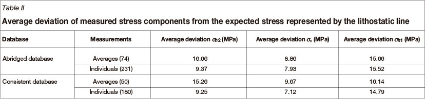
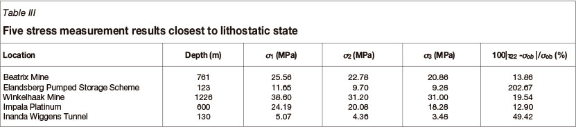
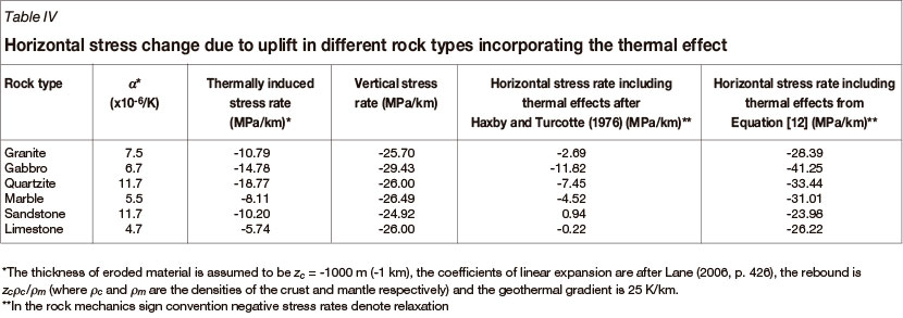
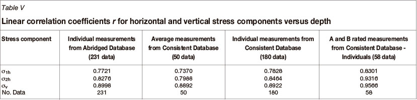
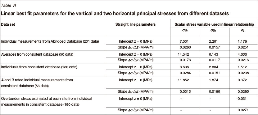