PAPERS

 

Singular value decomposition as an equation solver in co-kriging matrices

 

 

M. Kumral^I; P.A. Dowd^II

^IMining and Materials Engineering, McGill University, Montreal, Quebec, Canada
^IIThe University of Adelaide, School of Civil, Environmental and Mining Engineering, Australia

 

 

---

SYNOPSIS

One of the most significant elements in solving the co-kriging equations is the matrix solver. In this paper, the singular value decomposition (SVD) as an equation solver is proposed to solve the co-kriging matrices. Given that other equation solvers have various drawbacks, the SVD presents an alternative for solving the co-kriging matrices. The SVD is briefly discussed, and its performance is compared with the banded Gaussian elimination that is most frequently used in co-kriging matrices by means of case studies. In spite of the increase in the memory requirement, the SVD yields better results.

Keywords: co-kriging matrix, singular value decomposition, estimation/simulation.

---

 

 

Introduction

Any numerical analysis method, such as kriging or finite-element analysis, entails finding a solution, (x), for [A](x) = (B). The computation time for the solution increases as the dimension of [A] increases. Various equation solvers have been used in the co-kriging algorithms. The first published co-kriging program (Carr et al., 1985) used an iterative algorithm, which minimized memory use. It was easily adapted to equation solving when a sub-matrix structure existed. The method was called the algebraic reconstruction technique (ART). Because the algorithm was slow, a modified Gaussian elimination algorithm was then proposed. Carr and Myers (1990) pointed out that the sample-sample covariance matrix had the largest values on the diagonal. In the Gaussian elimination algorithm these diagonal values are used to normalize and reduce the matrix. In the co-kriging context, the diagonal entries in the sample-sample covariance matrix are matrices and thus the sub-matrix structure is generated. The sample-sample covariance matrix may be treated as a large matrix of scalar entries and reduced to the Gaussian elimination procedure. Similarly, the point-sample column vector is regarded as m column vectors, where m is the number of variables to be estimated. The vectors are individually reduced. Back substitution using each of the column vectors and the reduced covariance matrix yields a solution for the weights.

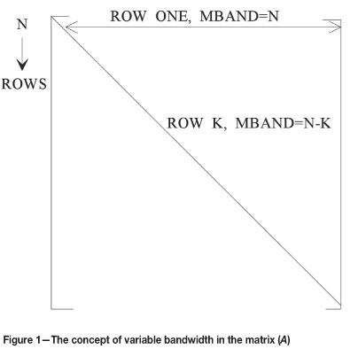
For the co-kriging matrix, the modified Gaussian elimination method was further modified to include the banded algorithm proposed by Carr and Myers (1990). This approach is inspired from the stiffness matrix in finite element analysis resulting from mesh design, in which node points are numbered most efficiently. Only a part of this matrix, a distance MBAND on either side of the diagonal, consists of non-zero entries. A reduction in computational time can therefore be obtained by using the MBAND portion above the diagonal and the diagonal itself in the calculation of the solution for (x). In kriging, the sample-sample covariance matrix is square, symmetric, and diagonal, as is the stiffness matrix. The banded-matrix concept is applied to the inter-sample covariance matrix by modifying the algorithm to allow a variable bandwidth (Figure 1).

 

 

Carr (1990) remarked that the variable bandwidth algorithm resulted in improved computational efficiency, especially as the number of nearest-neighbour samples used for estimation becomes large. The LU ecomposition produces a lower round-off error in comparison to the Gaussian elimination (Gomez-Hernandez and Srivastava, 1990). Table I shows a summary of the number of calculations associated with different equation solvers. Long and Myers (1997) noted that their co-kriging algorithm yielded poor estimates while generating maps. The size and sparsity of the co-kriging matrices inverted by the Gaussian elimination means that there is a very high risk of producing ill-conditioned matrices. Another important aspect is numeric precision, which has profound influence on co-kriging weights.

 

 

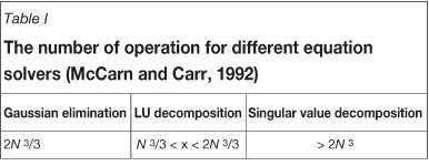
When the sample-sample covariance matrix is symmetric and diagonalized, the efficiency of the Gaussian elimination improved from 2N ³/3 to N ³/3. As can be seen from Table I, the Gaussian elimination and the LU decomposition methods have an advantage over the singular value decomposition (SVD) from the point of view of the number of operations. Some cases can attribute special importance to performance of the equation solver. For instance, while conditional distributions are extracted from ordinary co-kriging weights, co-kriging weights should be as accurate as possible, and also the sum of these weights should be exactly one (Rao and Journel, 1997). In this case, the SVD can be a good alternative for equation solving.

 

SVD for co-kriging matrices

The SVD is a powerful method for solving sets of equations or matrices. McCarn and Carr (1992) to some extent researched the method and pointed out that the SVD is identical in performance to the Gaussian elimination or the LU decomposition for the ordinary kriging context. However, the SVD has advantages and disadvantages in comparison to the Gaussian elimination and the LU decomposition:

Advantages:

1. In some cases where Gaussian elimination or the LU decomposition fail to give satisfactory results, especially in some spatial situations in which the matrix is close to singular, the SVD diagnoses and solves the matrix
2. In cases where the functions used to model the drift are not scaled properly in universal kriging, the SVD yields better results.

Disadvantages:

1. The SVD requires more computer time and memory
2. Because there are more numerical operations in the SVD, round-off error may be greater than in other methods. This may be controlled by using a small data set in the local neighbourhood or increasing the precision of the analysis.

In matrix algebra, linear equations may be solved for cases in which the matrix is non-singular. A kriging matrix comprises sample-sample and sample-point semivariogram values calculated from a semivariogram model. These values may be subject to experimental or observation errors, in addition to unavoidable round-off errors. A crucial question arises: how much is a solution altered by errors and how can the sensitivity of solutions to errors be quantified? In this situation, the SVD can diagnose the problem and yield a solution.

The SVD is based on the following theory of linear algebra. For any matrix A and any two orthogonal matrices U and V, consider the matrix W defined by:

If uj and vj are the columns of U and V, then the individual components of W are:

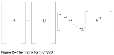
The idea of the SVD is that, by proper selection of U and V, it is possible to make most of the wj zero. In fact, it is possible to make W diagonal with non-negative diagonal entries. Consequently, a SVD of an M x N real matrix A is any factorization of the form:

where A is an M x N matrix, the number of rows (M) of which is greater than or equal to its number of columns N. A is said to be the product of an orthogonal matrix comprising Mx N columns, an N x N diagonal matrix W with positive or zero elements, and the transpose of an N x N orthogonal matrix V. The quantities wjof W are known as singular values of A, and the columns of U and V are known as the left and right singular vectors (Vetterling et al. 1993 and Press et al., 1992). Figure 2 illustrates the SVD in the matrix form:

 

 

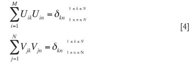
The matrices U and V are each orthogonal in the sense that their columns are orthonormal:

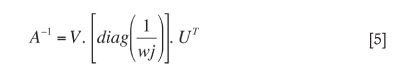
The inverse of matrix A is defined as:

The problem arises when one of the wi is zero, or very small, or is dominated by round-off errors. As the number of zero-valued wfs increases, the matrix becomes more singular. The SVD is able to diagnose kriging matrices by means of the decomposition shown in Figure 2.

The condition number of a matrix prescribes its singularity. The condition number is formally described as the ratio of the largest wj to the smallest wj. If the condition number of a matrix is infinite, the matrix is singular. In practice, whether a matrix is singular or non-singular is determined by its rank, but the determination is not easy. The columns of U whose same-numbered elements, wj, are non-zero are an orthonormal set of basis vectors that span the range. The columns of V whose same-numbered elements wi are zero are an orthonormal basis for the null space. To put it another way, if the matrix is diagonal, its rank is the number of non-zero diagonal entries. That is, the rank of the matrix A is the rank of the diagonal matrix W in its SVD. This observation determines whether kriging or co-kriging matrices are singular or non-singular, because being singular or non-singular means full rank or rank-deficient, respectively. With efficient rank the SVD works with the number of singular values greater than some prescribed tolerance which reflects the accuracy of the data. The great advantage of the SVD in determining the rank of a matrix is that decisions need be made only about the negligibility of single numbers rather than vectors or sets of vectors.

As mentioned earlier, it is common for some of the w/s to be very small but non-zero, which leads to ill-conditioned matrices. In these cases, a zero pivot may not be encountered with the Gaussian elimination or the LU decomposition. For Ax = b linear equations, the solution vector may have a large component whose algebraic cancellation may give a very poor approximation to the right hand vector b. In other words, a matrix is singular if its conditional number, expressed as the ratio of the largest of w/s to the smallest of w/s, is infinite. The closer the conditioning number approaches the computer's floating point precision of reciprocals (for instance, less than 10-6 for single precision or 10-12 for double precision), the more ill-conditioned the matrix becomes. In order to rectify this condition, these wj's are set to zero. Long and Myers (1997) showed that this diagnosis and solution was one of the most important advantages of using the SVD. The solution vector x obtained by zeroing the small w/s is better than both the direct method solutions and the SVD solution in which the small w/s are abandoned as non-zero.

In addition, provided some of the singular values are zero, fewer than N columns of U are needed. If K is the number of non-zero singular values, then U, W, and VT can be made M x K, K x K, and K x N respectively. Since they are not square, matrices U and V are not orthogonal. This version of the SVD might be called the 'economy size'. The saving in computer storage can be important if K or N is much smaller than M (Forsythe et al., 1977).

The choice of a zero threshold for small wfs is vital and may require experimentation. Apart from this, it is necessary to determine the size of the computed residuals (A. x - b) that is acceptable. In the subroutine, (Max (wj) x 10^-6) is used as the threshold (single precision).

Given the system A.x = b a linear system is expressed by the SVD:

and hence

where z = V^Tx and d = U^Tb. The system of equations wz = d is diagonal and hence can be easily solved. Depending upon the values of the dimensions m, n, and the rank k, the system separates the number of non-zero singular values into as many as three sets:

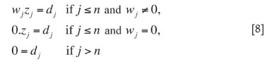
The second set of equations is empty if k = n, and the third is empty if n = m.

The equations are consistent and a solution exists if and only if dj = 0 whenever wj = 0 or j > n. If k < n, then zj associated with a zero wj can be given an arbitrary value and still yield a solution to the system. When transformed back to the original coordinates by x = Vz, these arbitrary components of z serve to parameterize the space of all possible solutions x.

 

Case study

Example 1

Using a data set of 200 samples, a domain was simulated at 625 locations for two variables. The simulations were implemented using both the banded Gaussian elimination and the SVD methods, and the performances compared. Sequential Gaussian simulation codes provided in the GSLIB (1992) were modified in co-simulation form. Banded Gaussian elimination and the SVD were then incorporated into the programming codes. The co-kriging weights for SVD totalled 1 for all simulated values. However, for banded Gaussian elimination, especially at the beginning of the procedure, the co-kriging weights deviated from 1. As all previously-simulated values are incorporated into the data set, the effects of the different weights produced by the two equation solvers are diminished and the kriging weights exhibit the same behaviour.

Semi- and cross-semivariograms used in the construction of case studies are illustrated in Figure 3.

 

 

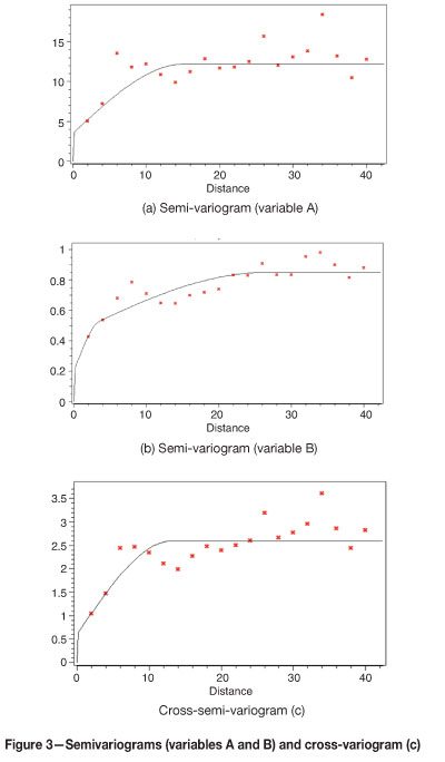
Table II shows the comparison of the results from the two equation solvers. It is assumed that the number and quality of declustered samples is adequate to represent the simulated field.

 

 

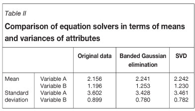
As can be seen, the SVD yields slightly better results than the banded Gaussian elimination. However, the SVD needs nearly twice more execution time than banded Gaussian elimination. As an alternative, both methods can be used in the algorithm in such a way that the SVD is used in at the beginning of the execution and is then followed by banded Gaussian elimination.

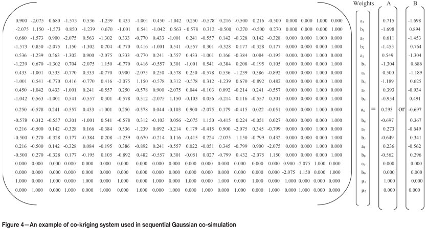
Example 2

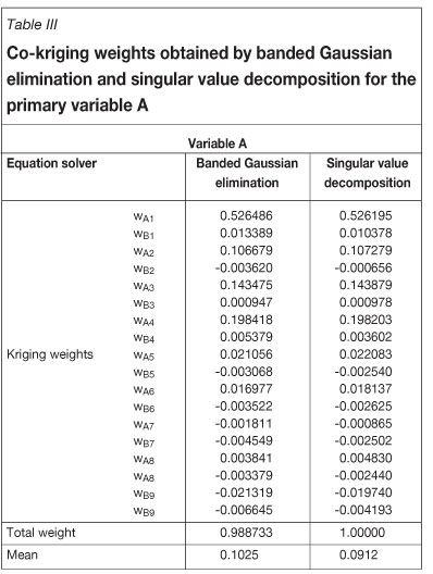
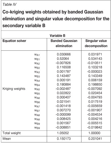
To further compare the performance of banded Gaussian elimination and SVD, the solution of the co-kriging system shown in Figure 4 is given for two variables at one of sequential co-simulation algorithm nodes. In the co-kriging system, co-located cross-semivariograms are used. The co-kriging matrix has been created by data values of the variables A and B from the eight closest sample points and simulated values of A and B from one previously simulation location (total 18 values). This example is selected from the beginning of the simulation (which is why only two previously, simulated values from one location are included in the data set) because the problem arising from the banded Gaussian elimination equation solver has been particularly observed at the beginning of simulation. The right hand side of the co-kriging matrix shows the covariance between data locations and the simulation location for variables A and B. As previously-simulated values are added to the data set, the Gaussian elimination and SVD yield the same kriging weights. As the problem is most pronounced at the beginning of a simulation, multiple realizations using different random paths is one solution for simulations at the first few nodes.

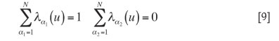
The ordinary co-kriging method was used in the algorithm, i.e., the sum of the weights assigned to values of the primary variable is set to 1 and the sum of the weights assigned to values of the secondary variable is set to 0:

As shown in Tables III and IV, the SVD yields kriging weights that sum exactly to 1 for both variables, while the sum of the kriging weights yielded by the banded Gaussian elimination method deviates from 1.

 

 

 

 

Conclusions

In this investigation, the performance of the SVD as an equation solver in co-kriging matrices was researched. This approach is valid only if co-located sample data is available -where all measurements are available on the same samples and the samples are ordered within the analysis so that all measurements on each sample are contiguous in the matrix expression of the equations to be solved. The SVD with double precision yields better results than the traditional methods of solving co-kriging equations, but requires more CPU time. Whereas banded Gaussian elimination completes 2500 simulation nodes in 5 seconds, the SVD completes the same number of nodes in about 10 seconds. As the number of simulations increases, the time involved in the use of the SVD may become prohibitive. As the matrix size increases, round-off errors increase. The neighbourhood size is an important variable in co-kriging algorithms. Maximum size of co-kriging has been limited to a maximum of eight data and eight previouslysimulated values in the example demonstrated in this paper. The problem resulting from the banded Gaussian elimination equation solver is particularly acute in the early stages of a simulation. As previously-simulated values are added to the data set, the Gaussian elimination and the SVD tend to yield the same kriging weights. Multiple realizations using different random paths provide an opportunity to observe the effects of the equation solver in the early stages of a simulation. The SVD can be used at the beginning of a simulation and the Gaussian elimination thereafter.

 

References

Carr, J. 1990. Rapid solution of kriging equations, using a banded Gauss elimination algorithm. International Journal of Mining and Geological Engineering, vol. 8. pp. 393-399.         [ Links ]

Carr, J., Myers, D.E., AND Glass, C.E. 1985. Cokriging- a computer program. Computers and Geosciences, vol. 11, no. 2. pp. 111-127.         [ Links ]

Carr, J. and Myers D. 1990. Efficiency of different equation solvers in cokriging. Computers and Geosciences, vol. 16, no. 5. pp. 705-716.         [ Links ]

Deutsch C.V., and Journel, A.G. 1992. GSLIB: Geostatistical Software Library and User's Guide. Oxford University. Press, New York. 340 pp.         [ Links ]

Forsythe, G.E., Malcolm, M.A., and Moler, C.B. 1977. Computer Methods for Mathematical Computations. Prentice-Hall, Englewood Cliffs, New Jersey. 259 pp.         [ Links ]

Gomez-Hernandez, J.J. and Srivastava, M. 1990. ISIM3D: an ANSI-C three dimensional multiple indicator conditional simulation program. Computers and Geosciences, vol. 16, no. 4. pp. 395-440.         [ Links ]

Long, A.E. and Myers, D.E. 1997. New formulation of the cokriging equations. Mathematical Geology, vol 29, no 5. pp. 685-703.         [ Links ]

McCarn, D.W. and Carr, J. 1992. Influence of numerical precision and equation solution algorithm on computation of kriging weights. Computer and Geoscience, vol. 18, no. 9. pp. 1127-1167.         [ Links ]

Press, W.H., Flannery, B.P., Teukolsky, S.A., and Vetterling, T.V. 1992. Numerical Recipes. Cambridge University Press. 818 pp.         [ Links ]

Rao, S.A. and Journel, A.G. 1997. Deriving conditional distributions from ordinary kriging. Baafi, E.Y. and Schofield, N.A. (eds.). Geostatistics Wollongong'96, vol. 1, pp. 92-102.         [ Links ]

Vetterling, T.V., Press, W.H., Teukolsky, S.A., and Flannery, B.P. 1993, Numerical Recipes. Cambridge University Press. 245 pp.         [ Links ]

 

 

Paper received Sep. 2011; revised paper received Apr. 2012.

 

 

© The Southern African Institute of Mining and Metallurgy, 2012. ISSN2225-6253.