TRANSACTION PAPER

 

Comparing two mass size distributions

 

 

F. Lombard^I; G.J. Lyman^II

^ICentre for Business Mathematics and Informatics, North-West University, Potchefstroom, South Africa
^IIMaterials Sampling and Consulting Pty Ltd, Southport, Australia

 

 

---

SYNOPSIS

We consider in this paper the use of a modified version of Hotelling's statistic in the analysis of particle size distributions. The statistic can be adversely affected by the presence of outliers among the data. We propose a competitor to the statistic that is based on ranks, and hence is less sensitive to outlier effects. The results of a Monte Carlo study suggest that the rank test is highly competitive with the Hotelling test in its ability to detect differences between two mass size distributions. The calculation of the rank statistic is explained in detail and its application is illustrated on two sets of data.

Keywords: mass size distributions, bias testing, rank statistic.

---

 

 

Introduction

Lyman, et al. (2010) reported in this Journal the results of research, both applied and theoretical, on the analysis of particle size distributions. The Hotelling T² statistic that was proposed can be adversely affected by the presence of outliers among the data. The paper promised further research into an improved methodology. In this paper we try to fulfil the promise. We propose a robust test procedure based on ranks as a competitor to the T² statistic. In a typical sizing procedure, a mass M kg of raw material is sorted into p + 1 size intervals (in millimetres)

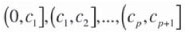
and the mass of material, M1,..., Mp+₁, in each of the size intervals recorded. Thus M = M₁+...+M_p+1. Often the value of M that is needed to achieve a target precision in sizing is suggested by an industrial standard (e.g. an ISO document) and is supposed to remain fixed over successive sieve analyses. In practice it is hardly possible to keep M constant, and deviations of a greater or lesser magnitude from the prescribed value occur as a matter of course. Consequently, the results of a sieve analysis are invariably reported as a vector of proportions x = (x₁,...,X_p+1), where

so that

As a consequence, the covariance matrix of the multivariate data set that results upon making n > d independent observations on the random vector x is singular.

In order to develop a statistical method to analyse such data, one thinks of the observation x = (x₁,...,X_p+1) as a corrupted realization of a 'true' underlying size distribution q = (q0,...,qp+i), Σqk = 1). The principal sources of corruption are mechanical sampling error and laboratory analysis error. Here qk denotes the true, but unknowable, proportion of the total mass of a large (conceptually infinite) amount of material that falls in the kth size interval. In this paper we consider tests of the hypothesis of equality of two such underlying size distributions. In the first of the two applications to be considered, two samples were obtained from the same batch of material, one by each sampling method, each sample having been sized using a set of p = 10 sieves. This pairwise collection and sizing of samples was repeated on n = 28 independent batches of material. Thus, we have 28 pairs

of observed sizings. The question is whether or not it is reasonable to assume that the distributions q underlying the x results are the same as the distributions q* that underlie the y results. We emphasize that the underlying size distributions typically vary from sample to sample because of the timewise variability in the supply of material being sampled. Thus we do not assume that the observation pairs (x¡, y₁), i = 1,...,28 are realizations of a fixed pair (q,q*) of underlying distributions. As such, an analysis should be based on the 28 sets of differences

Figure 1 shows for this data set boxplots of the 28 differences within each of the 10 size classes. Comparing the medians with the zero line, the overall visual impression is that the two size distributions differ somewhat. The sampler seems to be producing less coarse material, and consequently more of the finer material, than the stopped belt method. On the other hand, the Hotelling T² gives a non-significant result (p-value = 0.124), indicating, contrary to what we see in Figure 1, that the observed differences are nothing out of the ordinary. However, we also see that the data abound in outliers (the + signs in Figure 1) and that any real differences between the size distributions may have been masked by the large amount of variability in the data.

 

 

The main objective of the present paper is to demonstrate how outlier effects associated with the use of the T² statistic can be overcome. We will show that replacing the differences (Equation [4]) by appropriate rank scores takes care of the outlier problem without sacrificing much, if anything, in the ability to detect true differences (statistical power). A secondary objective of the paper is to show that the rank score test is, in fact, often more adept than Hotelling's T² at detecting real differences between commonly encountered size distributions.

The paper is structured as follows. We first review briefly the calculation and properties of the T² statistic in its application to sizing data. We then describe the rank score version of the statistic, illustrate its calculation on a small set of artificial data, and apply it to two real data sets. Following this, we use a Monte Carlo simulation method to compare the abilities of the tests to detect substantive differences between underlying size distributions. The results of the Monte Carlo study suggest that the proposed rank test is highly competitive with the Hotelling T² test. Finally, we make some concluding remarks and summarize our main results.

Hotelling's T² statistic

Set

and form the data matrix of differences

and the (column) vector of means

where k is the average of the n elements in row k of D. Lyman et al. (2010) proposed a procedure based on Hotelling's T² statistic to test the statistical significance of the observed differences ki by deleting any one of the rows of D, say the last one _p+1, and computing the T² statistic on the remaining rows ¹,...,_p. The T² statistic is

where

denotes the covariance matrix. The reason for eliminating one row of D from consideration is that the constraint Equation [2], which also applies to the j-data, together with Equation [5] implies that

so that the covariance matrix C is singular. This precludes calculation of T² on the full data matrix D. It is important to note that the numerical value of T² computed in the manner suggested by Lyman et al. does not depend upon which one of the p + 1 rows is eliminated from the data matrix. This fact is intuitively rather obvious because any p of the p + 1 rows contain the same information as does the full set of p + 1 rows—the missing row can be reconstructed exactly by applying the constraint (Equation [8]). Thus, the outcome of the statistical test is uniquely determined, no matter which one of the rows is eliminated from consideration.

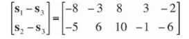
The following equally important fact will also be used in this paper. Namely, that for any data matrix, not necessarily constrained as in Equation [2], and row _l the numerical value of T² computed on the p nonzero row difference _k - l, k ≠ l does not depend upon l. For example, the numerical values of T² computed on the vectors

will be exactly the same. This follows from the fact that the numerical value of t² does not depend upon the ordering of rows in the data matrix D.

A rank test

A version of the t statistic that is robust to outliers is obtained upon replacing the differences _ik in row k of the data matrix by a rank score which is more or less immune to outlier effects. Towards this, notice that each _ik can be expressed as the product of its absolute value and its sign (+1 or -1),

In order to negate outlier effects one replaces | _ki I by its rank among the absolute values in row k,

Then, for example, the two largest absolute values in the row receive the ranks n - 1 and n, no matter how large they are compared to each other and to the other absolute values in the row. Appending the sign of _ki to its rank gives the rank score

Comparing Equations [9] and [10] we see that robustness is effected by the replacement of the numerical value of | ik |, which may be an outlier relative to the other | d | values in the row, with its rank, which is not an outlier relative to the other ranks in the row. In this way, each row dk = (ki,...kn) of the data matrix D is replaced by a row of rank scores sk = (s_k1,...s_kn) to form a new data matrix

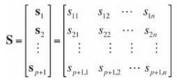
The proposed rank statistic, denoted by T²W, is obtained by choosing any one of the rows, say s_p+1, as a 'reference row' and calculating T2 t2 in Equation [6] on the reduced rank score matrix

The subscript w in t²_W serves to indicate that the rank scores are, in fact, those upon which the well-known Wilcoxon symmetry test is based. Notice that, in contrast to the _ki, the rank scores generally are not subject to the constraint . Hence, it would be possible in principle to compute  T²W on the full ranks score matrix S. This is not advisable, though, because near-singularity of the corresponding covariance matrix is a frequent occurrence and gives rise to unnecessarily variable T²_W values. Eliminating one of the rank score row vectors from the calculation is also not advisable.

This is because, in the absence of the constraint ^ski=0 the value of T²_W will then depend upon which score vector is eliminated. On the other hand, as was pointed out in the Introduction, basing the calculation on the reduced rank score matrix ensures a unique value of T²_W.

Numerical example

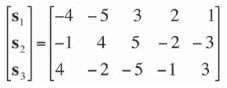
We illustrate the calculation of the rank scores on the following small set of artificial data:

Here, p = 2 and n = 5, that is, we have five paired sets of observations on each of three size fractions. The matrix of differences is

From this we derive the matrix of signs

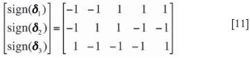
the matrix of absolute values

and the matrix of ranks

The rank score vectors are now found by multiplying corresponding elements of the matrices in Equations [11] and [12],

and the Hotelling statistic is computed on the matrix

or on the matrix

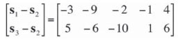
or on the matrix

The value of T²_W is 0.915 in all three cases.

A Matlab (Mathworks Inc., 2007) program that does the required calculations for data sets of realistic sizes is available from either of the authors upon request.

Application to sizing data

For the data set exhibited in Figure 1 the observed value of the T²_W statistic is 2.980 with a p -value of 0.022 found from the F distribution with 9 and 19 degrees of freedom. (The p -value is the probability that the T²_W statistic exceeds the value 2.98 given that it has the indicated F distribution.) This p -value of 0.022 is quite different from the p-value of 0.124 produced by the T2 statistic on this data. Thus, the rank test suggests strongly that the differences seen in Figure 1 are, in fact, real and not merely due to chance. Given this conclusion, an obvious question that arises is 'where do the differences mainly occur'? It was pointed out by Lyman et al. that some care should be exercised when attempting to answer this question. This is because a change in the mass fraction reported by any given size class must of necessity be accompanied by reported changes in one or more of the remaining size classes: the total of the reported fractions must be 1.00 under all circumstances. A glance at Figure 1 suggests that the reported proportions of coarser material (size fractions 7-10) have decreased while the proportions of finer material (size fractions 1-6) have increased correspondingly. This becomes clearer when we look at Figure 2, derived from Figure 1, which shows a plot of the medians of the 28 differences within each size class. Notwithstanding that the differences are relatively small, the pattern is clear.

 

 

Next, we turn to the data analyzed by Lyman et al. (2010) . This involved a comparison of sizings from samples of iron ore obtained with two different cross-belt samplers, a Vezin-type belt-end sampler, and stopped belt sampling. A total of 14 pairs of sizings into 8 intervals from each procedure were available for analysis. Belt sampling was carried out by highly experienced staff and sample analysis (sizing) by a well-accredited laboratory that was closely supervised. The reproducibility of the sizing protocol was established prior to processing the test samples. Figure 3 (which is a reproduction of part of the top left hand one in Figure 3 of Lyman et al. (2010), except that the size fractions are now arranged left to right from finest to coarsest, shows boxplots of the 14 differences in each of the 8 size intervals for the belt-end sampler and the stopped belt samples. Student t -tests comparing each of the size fractions indicated a significant difference at only the finest size fraction. (We point out here that in Table 1 of Lyman et al. (2010) the numbers 0.160, 0.25, 2.68, and 0.64 in the last row of the belt-end block should be replaced by 0.887, 0.162, 14.6, and 5.48 respectively.) The Hotelling T also indicated an overall significant difference (p -value = 0.05). Since a bias from cross-stream (Vezin) sampling was somewhat unexpected, the question was put whether outliers (indicated by a + in Figure 3) could have been the cause of the significance of the values of the t and T2 statistics. The answer seems to be that the observed differences are real—the rank test also gives a highly significant result for these data (p -value = 0.003). Some confirmation that the highly significant T2 and T²_W values are at least in part due to the observed differences in the finest size fraction follows upon analysing the subcompositions (x²ⁱ,..X⁸ⁱ) / (1 -x¹ⁱ) and (j²ⁱ,-,y8⁷ⁱ) / (1 -y¹ⁱ) consisting of the size fractions in intervals 1 through 7 only. Then neither T2 nor T²_W is significant (p-values of 0.54 and 0.31 respectively).

 

 

 

 

Technical note

The F-distribution with p and n-p degrees of freedom attributed to the T² statistic and which is used to determine significance levels, requires a formal assumption that the matrix of differences originates from an underlying multivariate normal distribution. This assumption is hardly likely to be satisfied for sizing data, particularly since the entries in the vectors _k must all lie between -1 and +1. Nonetheless, extensive simulation results, some of which are reported in the next section, indicate that the F -distribution can be safely used. This can be explained partially by noting that the T² statistic depends on the raw data only through the mean vector and the covariance matrix C, both of which are averages computed from the differences; see Equations [5] and [7]. Now, the central limit theorem guarantees approximate normality of averages, especially for difference data such as k - l that are constrained to lie in a finite interval and that do not exhibit an excessively skewed distribution. Thus, it is perhaps not so surprising that the F -distribution is applicable to the data that we are dealing with, even when only relatively small amounts of such data are available.

Monte Carlo simulations

In this section of the paper we present the results of some Monte Carlo simulations with a view to (i) demonstrating the applicability of the F distribution when determining significance levels and (ii) comparing the statistical power of the rank test with that of the Hotelling test. The power of a statistical test (or a test statistic) is defined as the probability that the test will succeed in identifying a difference that is indeed present. A test with a power of 1 (or 100%) 'never fails'.

One approach towards these goals is to generate artificial data sets based on models that attempt to simulate the mechanisms that lead to an observed size distribution, such as particle breakage and particle sampling error (Brown and Wohletz (1995); Dacey and Krumbein (1979); Gy (1982); Lyman (1986)). However, since we have a number of real data sets at our disposal, we prefer to base our simulations directly on these.

In order to judge the applicability of the F distribution we require pairs of observed sizings that are generated from the same underlying size distribution and which differ only in respect of uncertainties added in the sampling and sieving operations. Given a data set consisting of n pairs of observed sizings (columns) (x¡, y_i), i = 1,...,n, data sets with the required structure can be generated by interchanging at random the roles of xi and yi in the data matrix. That is, we flip an unbiased coin and if it shows heads we replace the pair (x¡, y_i) by (y_i, x_i) in the data matrix, otherwise leaving it unchanged. This means that we are sampling at random from a large collection of 2ⁿ pairs of data sets of which any pair of columns is generated from identical underlying size distributions (the size distributions may vary from column pair to column pair). In the numerical example given earlier (n = 5), suppose five coin flips resulted in the outcome H, T, T, H, T

Then the corresponding randomized data matrix would be and the Hotelling and rank statistics would be computed on this data matrix in the manner indicated in the numerical example given earlier. This generation of randomized data sets is repeated a large number of times, say N times. We then compute the observed fractions of these N times in which each of the two statistics exceeded the upper 100 (1 - a)% percentile c_a of the F distribution with p and n - p degrees of freedom. If the F distribution is applicable, the fractions should be close to a. Table I shows the results obtained when applying this method to the data in Figure 1 (n = 28) and Figure 3 (n = 14) using in each instance N = 50 000 trials and a = 0.10, 0.05, and 0.01. Clearly, the empirical exceedance probabilities of the rank test are quite close to the nominal values in all cases while the Hotelling statistic seems to undershoot the mark slightly.

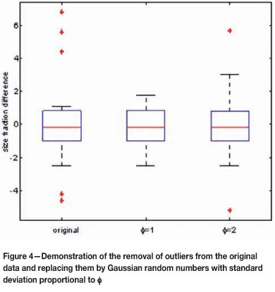
To gauge the effect of outliers on the tests we again use the data from Figures 1 and 3, but now in a different manner. We replace in each interval those observed size fraction differences d_ki that were identified as outliers by pseudo observations constructed as follows. Denote by iqr the interquartile range of the data in row k and denote by m their median. A Gaussian distribution of differences without outliers in row k would have a mean equal to m and a standard deviation equal to 0.69 x iqr. Notice that 0.69 is the ratio between the 68th (median + one standard deviation) and 75th percentiles of a Gaussian distribution. Each outlier in row k is now replaced by an observation from a Gaussian distribution which has mean m and standard deviation F x 0.69 x iqr. Here, ^ is a variance inflation factor. The data set thus reconstructed has exactly the same configuration of median differences as the original. When F = 1, all outliers have essentially been removed. If F is increased, more outliers are artificially introduced.

We illustrate the procedure using the data in the eighth size interval in Figure 1 . There are five outliers, namely -0.046, -0.042, 0.044, 0.056, and 0.068. The median and iqr of the differences in row 8 are -0.002 and 0.019 respectively. A Gaussian distribution with this median and iqr would have a mean of -0.002 and a standard deviation of 0.69 x 0.019 = 0.013. Accordingly, with Ф = 1 we generate five such Gaussian random numbers and insert them into column 8 in place of the original five outliers. If Ф = 2, we replace the outliers by five random numbers from a Gaussian distribution with mean -0.002 and standard deviation 2 x 0.013 = 0.026, etc. Figure 4 shows boxplots of the original data and those that resulted from one application of the above procedure at Ф = 1 (the pseudo observations were -0.022, -0.011, 0.010, 0.017, 0.018) and Ф = 2(the pseudo observations were -0.050, -0.022, 0.008, 0.031, 0.057). We see that there are now no outliers at Ф = 1and just two at Ф = 2.

 

 

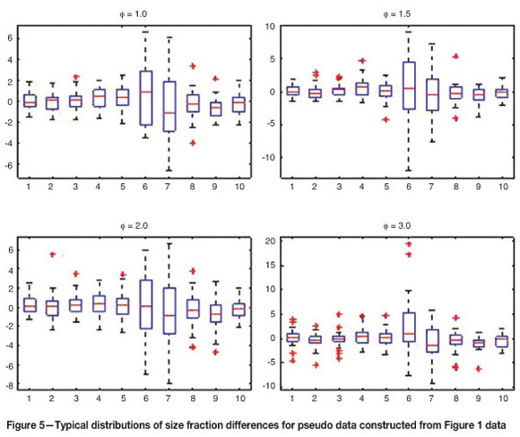
As Ф increases, so does the number of artificially generated outliers. Of course, after adding the perturbed values, we subtract from each column of differences its average in order that the necessary constraint be satisfied for the new data. This process of replacing the original outliers is repeated N times for each of a range of values of Ф. Then we find the fractions of the N times in which each of the statistics exceeds c_a. These fractions are our estimates of the statistical powers of the tests. (Needless to say, this will be a fruitless exercise if neither of the tests gave a significant result on the original data set.) Table II shows the estimated powers of the tests when this methodology is applied to the data from Figures 1 and 3 with a = 0.05 and N = 10 000. Figure 5 shows for each value of 4 in the first line of Table II (data from Figure 1) a boxplot of one randomly generated set of pseudo differences. Figure 6 shows the same in respect of the 4 values in the fourth line of the table (data from Figure 3). A general conclusion from these simulation results is that the T2 and T ² statistics have similar powers when the numbers and sizes of outliers are not extensive, but that the former statistic loses power much more rapidly than the latter as the numbers and sizes of outliers increase. Overall, it would seem that the rank test is to be preferred because of its greater power robustness.

 

 

 

 

 

 

Concluding remarks

The data used in this study to illustrate the virtues of the ranked score version of the Hotelling procedure by comparison to those of the conventional Hotelling test are real, and reflect the realities of bias testing using size distribution data. This contribution to the tools for making bias tests is motivated by the need to ensure that such tests are evaluated using the most powerful statistical tools.

However, it is critical in bias testing that the magnitude of the detectable bias be economically relevant. That is, the testing protocol, which includes sample masses collected, precision of the particle sizing process, the number of paired samples collected, and the statistical analysis procedure must be adequate to detect a difference between the test samples and the reference samples that is economically significant. Too often, a bias test is carried out using the guidelines provided by a standard. The accuracy of the work carried out is not specifically assessed and so the extent of the detectable bias is not quantified. A bias test which is not qualified by the extent of the detectable bias is no test at all, and may give comfort where none is to be had. Bias tests must be designed to detect a certain level of bias that has been based on an economic evaluation of the critical level of bias to be detected for all analytes of interest. Consideration of the size-by-size analyses of the material sampled for all economically important analytes, coupled with a critical consideration of the contractual tolerances on analytes, can be used to arrive at the critical level of bias to be detected in a test.

The authors continue to work towards a workable methodology for accurate assessment of the detectable bias over the full sizing distribution.

 

Summary

In this paper we propose a robust procedure based on ranks to test for sizing bias in a mechanical sampling system. The data consists of observed mass size distributions and our results are applicable to such data in general. The proposed rank test has been applied to two data sets and its advantages over Hotelling's T² statistic has been illustrated in a Monte Carlo simulation study using a very realistic method of injecting outliers into the data set. In particular, and in contrast to the T² statistic, the power of the rank test is not unduly affected by the presence of outliers. Our simulation results indicate that use of the F -distribution to compute p -values is permissible, even if relatively few sizing pairs are available. The testing carried out in this paper clears the way for the ranked Hotelling test to become a reliable standard tool in size distribution comparison, which comparison is a best tool for bias testing of sampling systems.

 

References

1. BROWN, W.K. and WOHLETZ, K.H. 1995. Derivation of the Weibull distribution based on physical principles and its connection to the Rosin-Rammler and lognormal distributions. Journal of Applied Physics, vol. 78, no. 4. pp. 2758-2763.         [ Links ]

2. DACEY, M.F. and KRUMBEIN, W.C. 1979. Models of breakage and selection for particle size distributions. Mathematical Geology, vol. 11 . pp. 193-222.         [ Links ] Gy, P.M. 1982. Sampling of Particulate Materials—Theory and Practice,

3. ELSEVIER, NEW YORK. LYMAN, G.J., NEL, M., LOMBARD, F., STEINHAUS, R., and BARTLETT, H. 2010. Bias testing of cross-belt samplers. Journal of the Southern African Intitute of

4. MINING and METALLURGY, vol. 110, no. 6. pp. 289-298. Lyman, G.J. 1986. Application of Gy's sampling theory to coal: A simplified explanation and illustration of some basic aspects. International Journal of Mineral Processing, vol. 17. pp. 1-22. Mathworks Inc. 2007. Matlab, Version 7.5 (release 2007b). ♦

 

 

Paper received Jul. 2011
Revised paper received Nov. 2011