JOURNAL PAPER

 

A case study application of linear programming and simulation to mine planning

 

 

J.A. de Carvalho Junior^I; J.C. Koppe^II; J.F.C.L. Costa^II

^ICopelmiMineração LTDA, Porto Alegre, Brazil
^IIMining Engineering Department, UFRGS, Porto Alegre, Brazil

 

 

---

SYNOPSIS

This paper analyses the impact of the uncertainty associated with the input parameters in a mine planning optimization model. A real example was considered to aid in the building of a mathematical model that represents the coal production process with reference to the mining, processing, and marketing of coal. This model was optimized using the linear programming concept whereby the best solution was perturbed by the stochastic behaviuor of one of the main parameters involved in the production process. The analysis of the results obtained permitted an evaluation of the risk associated with the best solution due to the uncertainty in the input parameters.

Keywords: mine planning, optimization, risk analysis.

---

 

 

Introduction

Although coal accounts for approximately 50 per cent of the national reserve of fossil fuel, its use in Brazilian energy generation has fallen continuously in the last few years, and coal now contributes less than 1.5 per cent to the total consumption of fossil fuels. This has prompted mining companies to diversify their customer base by supplying thermal coal to other industries such as the petrochemical, ceramic, paper, and cellulose industries, where coal is used for the generation of heat, steam, and/or electrical power for industrial plants; the food industry, where coal is used in the process of drying food grains; and the cement industry, where coal is used in the clinker mix in the kilns.

This diversification has forced the mining companies to develop new products to meet the specific needs of each customer. Companies that produced thermal coal with a calorific value ranging from 3 000 to 4 500 kcal/kg in the past, with practically no restrictions on the sulphur content, have had to increase their range of products. Nowadays, the local market for industrial-purpose coal demands products with higher calorific values (4 700 to 6 800 kcal/kg) and a lower sulphur content (usually below 1.2 per cent). In this context, and with the constant expansion of the global economy, local coal-mining companies are continually looking for alternatives that facilitate the production of better products with competitive prices in comparison with other energy-yielding products such as natural gas, fuel oil, and imported coal. An additional complexity is added to production planning by the fact that major coal producers frequently operate multiple mines with multiple pits feeding multiple processing plants within these mines.

The alternatives commonly chosen to attend to multiple customers in this multiple-option production scheme include the following:

(i) Simultaneously mining multiple mines, multiple pits, and multiple benches (seams) to increase the availability of run-of-mine (ROM) coal with different characteristics

(ii) Washing of coal from each seam separately to enhance the yield at the plant and approximate the characteristics of the washed coal to the desired final product

(iii Minimizing the mining dilution so that the characteristics of the ROM coal are as close as possible to the final saleable product.

The definition of the production strategy to meet a certain market demand is usually achieved by testing a few production scenarios: the finally chosen method should generate the highest economic benefit. However, this methodology does not guarantee that the chosen solution is really the best possible one. With the use of linear programming, it is possible to find the best production strategy to meet the demand of each market.

This problem can be tackled from an operational research (OR) perspective. An adequate thermal coal can be produced with a minimum cost and/or with a higher possible profit. The production depends on a variety of parameters and restrictions such as raw material availability, coal quality (different coal seams), specific product requests, recovery in the processing plant (which depends on the raw material used and on the characteristics of the desired product), and the mining and processing costs. These parameters specify the production of coal within certain limits.

There are various models and mathematical programming tools for solving this kind of problem. Among the several optimization techniques developed, the linear programming (LP) method has been the most studied, and hence the most widely used in several of the applied sciences. LP is not only the simplest technique in mathematical programming, but also the most versatile, offering the possibility of analysing the appropriateness of the chosen model concurrent with a guarantee for obtaining its global best, if it exists.

Due to their complex behaviour, some of the process parameters, can be regarded as stochastic. To quantify the impact of these parameters on the optimized outputs derived from LP, simulation techniques can be used, taking into consideration not only the averages or the deterministic patterns, but also the statistical distributions of the parameters considered.

This paper introduces a methodology for evaluating the impact of the uncertainty associated with input parameters on a given objective function using an optimization program that is based on LP. A case study concerning a major Brazilian coal-producing company illustrates the process by which the economil benefits of using the optimal solution are evaluated in comparison with the solution conventionally used by this particular mining company. Moreover, incorporating the uncertainty associated with the input parameters permits an assessment of the risk in reaching or not reaching the optimized solution.

 

Model of linear programming

According to Prado¹, LP is a technique that allows the merging of several variables on the basis of a linear function of effectiveness (objective function) while simultaneously satisfying a group of linear restrictions for these variables. The construction of a LP model follows three basic steps (Ravindran et al.²):

(i) Identifying the unknown variables to be determined and representing them using algebraic symbols

(ii) Listing all the restrictions of the problem and expressing them as linear equations in terms of the decision variables defined in the previous step

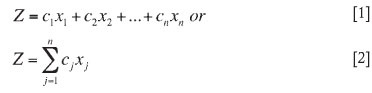
(iii) Identifying the objective or criterion for optimizing the problem and representing it as a linear function of the decision variables. The objective can be either a maximizing or a minimizing function.

Given an LP problem consisting of many variables in the maximization or minimization mode from a specific linear function, which is also known as the objective function (OF), the variables are submitted to a group of restrictions that are also linear. Generally, a problem in LP is formulated as follows. The restriction of 'no negativity in the decision variables' constitutes a necessary condition for the application of the solution algorithm. Although this restriction usually holds good due to the nature of the variables used in the model, under certain circumstances it can lead to situations where the variables become unrestricted. In this situation, an artificial variable should be used to substitute each unrestricted variable by the difference between the other two variables for which the restriction of 'no negativity' is applied (Loesch and Hein³).

Briefly, the algorithm can be described as follows: (i) Maximize or minimize the OF of the type or

(ii) Submit the variables to the following restrictions:

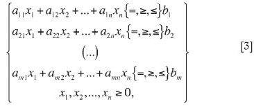
Where x_n are the decision variables, c_n are parameters of the OF, a_mn are parameters of the restriction equations, b_nn is an independent term of the restriction equations, n is the number of decision variables, and m is the number of functional restrictions.

The values of all the coefficients, or control parameters, are known during the modelling of the problem. These coefficients can have either deterministic or probabilistic characteristics depending on the nature of the problem modelled (Montevevechi⁴).

 

Algorithms for the solution

The simplex method is the algorithm typically employed in the solution of linear programming problems (LPPs). This technique uses the available tool in linear algebra to determine the best solution for the LPP by an algebraic iterative method.

Generally, the algorithm is created by a viable solution of the system of equations that constitute the restrictions of LPPs, and starting from that initial solution, it identifies either new viable solutions for the same or a better value for the problem than the current one. The algorithm, therefore, possesses (i) a choice criterion that provides the opportunity for always finding new and better vertexes of the convex boundary of the problem, and (ii) a stop criterion that can verify whether the chosen vertex is the one giving the optimum solution (Goldbarg5).

The basis for the simplex algorithm is in the formatting of the limited area for the restrictions, common in all OR problems (Dantzig⁶). Such an area is called simplex. Any two points selected in the outline of a feasible region, when united by a line, result in a line positioned entirely inside the simplex. Starting from the verification, the search for the solution in OR problems becomes limited to the extreme points of the simplex area. This observation has facilitated the development of an algorithm of low computational complexity for solving this problem by Dantzig⁶.

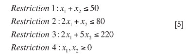
The algorithm of LP can be explained using a simplified graphical sketch; however, the illustration is limited to two decision variables. The example used to illustrate the method uses the following OF:

The OF is subjected to the following restrictions:

After plotting the lines corresponding to the above restrictions, an area within which all restrictions are simultaneously satisfied (hatched region in Figure 1) is defined. The polygon defined by the corners A, B, C, D, and E is known as the 'admissible region'.

 

 

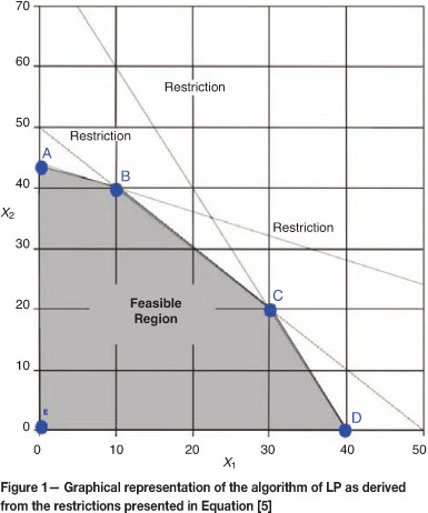
To define the optimum solution, the line corresponding to the OF, for a specific value of Z, is initially plotted. In the next step, various values are defined for Z, and the OFs for each defined Z are plotted. A group of parallel lines, known as the lines of the OF levels, is obtained (traced red lines in Figure 2). The OF grows towards the direction of its gradient (arrow in Figure 2), and the optimum solution is obtained at the maximum OF that intersects the feasible region.

 

 

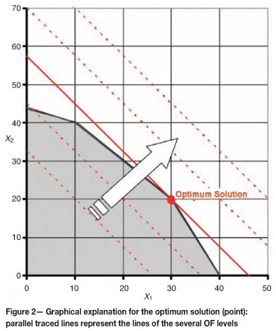
In a two-dimensional solution, the feasible region is shown in plan. The equation that represents the OF can be depicted by a vector, so that it is possible to reach the highest point by following the direction of improvement of the OF as determined by the vector inside the space of feasible solutions. The search guarantees that (i) one of the extreme points respectively maximizes or minimizes the OF, and its value is the maximum or the minimum, respectively; (ii) once the search for the highest point is restricted to the space of viable solutions of the problem, the optimum vertex satisfies the group of restrictions composing the problem of LP (Fogliatto⁷).

This reasoning can be extended to problems of larger dimensions. Bazaraa⁸ establishes that while searching for the highest point during the tracking of the space of viable solutions for an LP problem, the solution should correspond to one of the extreme points of the simplex. In practice, this can correspond to a point, a straight line, a plan, or any other pattern with a larger dimension.

The detailed mathematical presentation of the simplex algorithm can be found along with practical examples in most of the articles referring to LP; see, for example, Ravindran et al.², Loesch and Hein³, Goldbarg⁵, Dantzig⁶, Bazaraa⁸, and Bronson⁹.

 

Stochastic simulation

While creating a representative model of any industrial process in which the behaviours of all the parameters are not perfectly known, it is not possible to be certain about the results generated by the model. However, it is always possible to use methodologies of risk analysis to mitigate the effects of the uncertainty and to visualize the risk problem (Motta¹⁰).

For each group of restrictions that encircle the problem, a group of answers can be obtained from the model using simulation techniques to imitate the stochastic behavior of the process parameters that are not deterministic. This group of answers can be associated with the uncertainty space and can be used to quantify the inherent risk of the given process.

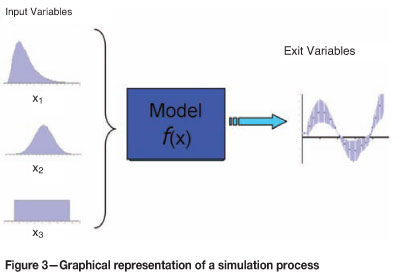
According to the functional visualization proposed by Menner¹¹, in simulation studies, the models possess (i) a number of entrances or inputs x₁, x₂,..., xr; (ii) a number of parameters related to the system p₁, p₂,..., pt; and (iii) a number of exits or results y₁, y₂,..., ys, which are the results defined by a function of the type f (x, y).

Simulation in the sense used in this study constitutes some mathematical techniques used to mimic any type of real operation or process (Freitas¹²). There are a few other definitions for the term 'simulation'. According to Schriber¹³, simulation in modelling implies a process or system that imitates the responses of the real system during a succession of events occurring over an extended period.

Pegden et al.¹⁴ present a more comprehensive definition of the simulation process. According to these authors, a simulation should fulfill the following objectives:

(i) Describe the behaviour of a certain system

(ii) Help in building a theoretical framework and explain an arbitrary hypothesis, given the observations provided by the simulation model

(iii) The model finally adopted should be able to predict new responses due to either a modified system or modifications in the production processes.

Contrary to the optimization methods, simulation does not yield an optimal result. Simulations provide a set of responses for a certain group of variables that condition the system (Figure 3).

 

 

The main advantages of a simulation process include the following (Pegden et al.¹⁴; Banks and Carson¹⁵):

(i) Simulation is simpler to use than an analytical solution

(ii) Although analytical optimization models normally require many simplifications to obtain a treatable solution, simulation models do not require these simplifications

(iii) Any hypothesis about how certain variables influence the system can be evaluated using the simulation model

(iv) An appraisal of the variables that are more relevant to the performance of the system and details of the interaction between the input variables leading to a certain response becomes possible

(v) New variations in the production process can be screened before practical implementation and their performances can be assessed.

Some systems do not show any probabilistic variables and hence are known as deterministic. In these circumstances, the responses are conditioned only by the input variables and their interrelations. In various situations, the input Variables system is controlled by random input variables and, consequently, a stochastic simulation is used to obtain the response of the system to a set of inputs. In this latter situation, the responses are also variable and are modelled using a probability function.

In the following section, a simulation model is presented that mimics the production process of thermal coal. The model is constituted by the following factors: (i) the input variables, x: the amount of ROM coal originating from different seams or mines; (ii) the parameters of the system, p: the operational cost associated with the mining and processing of the ROM, the indexes of recovery in the improvement process, and the selling prices of the different products; and (iii) the exit variables, y: the cash flow and the values of the liquid assets available. In these terms, the two groups that contain the input variables and the parameters of the system comprise the elements associated with uncertainty, and these can therefore be treated as random variables.

 

Settings, products, and production routes

Similar to other mineral commodities, coal production can be divided into two main stages: exploitation and processing. Coal mining occurs by open-pit mining, whereby the topsoil and other sedimentary formations that cover the coal seams, constituting the overburden, are stripped first, uncovering the coal seams underneath; these are later mined in an individual and selective manner (Hartman¹⁶). Generically, the mining operation involves the production of large amounts of waste material for each ton of coal extracted, constituting one of the more costly operational stages of the productive process.

The case under consideration is at Copelmi Mineração Ltda. Copelmi is the largest private coal-mining company in Brazil, supplying 80 per cent of the industrial market and 18 per cent of the total Brazilian coal market. Its facilities are located at Rio Grande do Sul State, in the southernmost part of the country.

The company currently operates four coal mines, commercializing approximately 1.5 Mt of coal per year. Its flexibility in producing at multiple mines enables a diverse product range with calorific value products ranging from 3100 kcal/kg up to 6000 kcal/kg.

Copelmi's main products are steam coal for a power plant, a petrochemical plant, and a large paper mill, all located within a maximum distance of 150 km from the mines.

During the period analysed, four mines were under simultaneous operation: Recreio Mine, ButiáLeste Mine, Faxinal Mine, and the Cerro Mine. Each mine exploited a number of coal seams with different qualities and reserves.

After the mining stage, the coal from the mines is transported to a washing plant, where it is processed to obtain a saleable product. The coal from each mine is processed at the closest washing plant. During this processing stage, impurities such as pyrite and clay present in the ROM coal are removed to reduce the emission of ash and gas during coal combustion. When the mine production exceeds the feed capacity of the plant due to any operational contingency, the excess ROM is diverted to the stockpile for future use. The washing process yields several types of products. The different production strategies are explained in the specifications of the OF section of the paper.

One of the most relevant operational parameters in the washing process is the yield or recovery. This parameter corresponds to the ratio between the amount of product generated and the amount of ROM coal fed into the plant, which may be stated as follows:

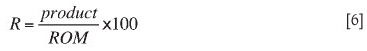
Where R is the yield (%), Product is amount of product generated (t), and ROM is amount of run-of-mine coal fed into the washing plant (t).

In addition to the product, the washing plant generates tailings, which are disposed at the tailings dam. These tailings are predominantly composed of clay and pyrite; however, due to the inefficiency of the processing plant, organic matter can be added to the tailings. In the latter instance, depending on the ash content of the tailings, the tailings can be redirected to be blended with other products.

 

Mathematical modelling of the production process

The central subject of the mathematical modelling is the description of the production process and its decision variables. The quantity (in tons) to be extracted and processed from each seam can be determined, thus fulfilling the demand for each product commercialized by the company. Optimization is achieved when the production process generates the largest possible operational contribution after abiding by all the restrictions imposed on the production process, in addition to considering the demands of the consumer market.

The decision variables are defined as follows:

Qij: amount of ROM coal of j seam extracted from mine i

E_ji amount of ROM coal of j seam used (or added) from the stock of mine i

A_jilk: amount of ROM coal of j seam extracted from mine i and processed by the washing plant to obtain a product k.

The process parameters are, among others: coal yield (plant recovery), production costs, selling prices of the products, and the tonnage and quality of the product specified by the consumers.

Objective function

Once the decision variables are defined, the next step is the definition of the OF. This function is represented by Equation [7], and its goal is to maximize the operational contribution satisfying a certain market demand.

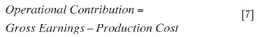
The operational contribution is the financial result obtained by the commercialization of the generated products (gross earnings), except for the costs exclusively associated with the production process (production costs) (Equation[7]).

This function can be better understood if it is subdivided into four corresponding portions: mining costs (MC), costs of stocks (SC), washing costs (WC), and gross earnings (GE). For this variant, a series of parameters representing the economical, operational, commercial, and geological factors are used, which can present either deterministic or probabilistic behaviours depending on the methodology used. The four portions that constitute the OF can be expressed in the form of Equations [8] to [12].

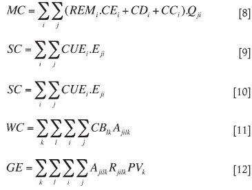
Where: i = index of the mines; j = index of the seams; l = index of the improvement plants; k = index of the generated products; REM_i = stripping ratio of mine i (m³/t ROM); CE_i = cost of waste removal from mine i (R$/m³); CD_i= blasting cost of mine i (R$/t ROM); CC_i = cost of extraction and transport of coal from mine i (R$/t ROM); Q_ji = amount of coal from seam j extracted from mine i (R$/t ROM); CUE_i = cost of handling unit stock of ROM coal in mine i (R$/t ROM), E_ij = amount of ROM coal of seam j moved on the basis of the stock of the mine i (t ROM); CB_lk = processing cost of ROM coal in the washing plant for the production of substance k (R$/t ROM); A_jilk = amount of seam j of mine i fed and processed in the washing plant to obtain product k (%); Rjilk = yield from seam j of mine i processed in washing plant to obtain product k(%); and PV_k = selling price of the product k (R$/t).

Restrictions

The restrictions defined in the outline conditions form the system and define the domain of the possible values for the decision variables. In the current case study, the group of restrictions comprises the following:

Geological proportion of the seams (percentage of seam j in the total quantity mined) in each mine

Maximum capacity of ROM coal production from the mines

Maximum coal tonnage able to be fed into each washing plant

Recovery of each product at each washing plant

Market demand

Qualitative/quantitative restrictions.

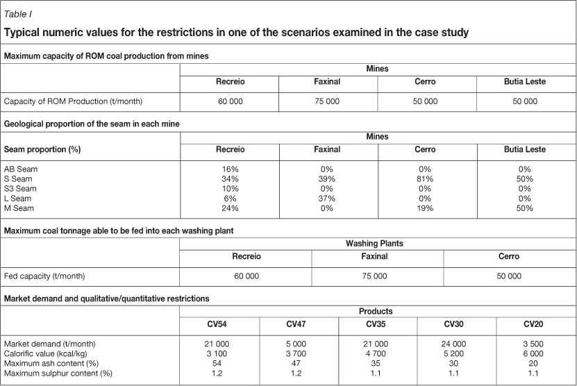
Table I shows typical numeric values for the restrictions in one of the scenarios examined in the case study.

This group of restrictions defines a mathematical formulation formed by 64 linear equations represented in terms of decision variables. The theoretical background and the mathematical formulation used to represent the group of restrictions in this case study are found in Carvalho¹⁷.

An optimization model composed of both the OF and the group of restrictions after considering the simplifications detailed above was implemented using Excel^®, using the educational version of the program 'What's Best^® 7.0' as an optimizer (Lindo Systems¹⁸).

 

Results of optimization

The outputs generated by the optimization model have been analysed, taking into account the different production scenarios. The production scenarios correspond to the monthly production strategy adopted by the company in 10 different periods during the years 2004 and 2005.

The results are analysed in two steps: the first quantifies the earnings that would be obtained by using the optimization model, and the second verifies the risk associated with each production scenario, considering that the parameters corresponding to the yield (coal recovery at the washing plant) behave stochastically, not deterministically.

Analysis of the responses

To quantify the earnings that an optimization model can generate in the production process, a comparison of the financial results obtained from the optimization model with those obtained in the same period adopting the non-optimized production scheme was conducted. The production strategy proposed by the mine planning staff without using optimization tools was adopted as the benchmark.

The scenarios chosen for comparison correspond to the production strategy adopted by the company in 10 different situations during the years 2004 and 2005. These situations, denominated 'Scenario 1' to 'Scenario 10', represent conditions where the market or the operation caused a significant change in the baseline conditions that define the production strategy of the company.

The optimization process yields as the final result the OF and the production strategy that need to be adopted. These strategies correspond to the amount of coal that should be extracted from each mine, its destination in terms of the processing plant, and the seam that provides the highest value for the specific OF.

To quantify the earnings that the optimization process can generate in a non-optimized process, the final results of the OF obtained from the optimization model were compared with the final results obtained following a non-optimized practical planning process adopted by the company, subject to the same conditions. The relative differences in the values of the OF for each of the 10 tested scenarios are presented in Figure 4.

 

 

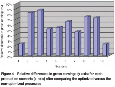
Figure 4 portrays the results for 10 production scenarios, with a minimum increase of 2.2 per cent and maximum of 8.7 per cent in the gross earnings, when the optimized scenarios are compared with the respective non-optimized procedures adopted by the company. An important practical aspect that needs to be pointed out is that this gain in earnings can be obtained by optimizing the production process within its operational limits, without the need for any additional investment in the process.

In addition to measurable gains as described previously, the use of an optimization model provides greater flexibility in the decision-making process. The method provides the resource to analyse the impact of possible changes in the production process, such as changes in the quantity of product sold and increase or decrease in the production costs.

Risk analysis of the optimization model

An optimization model as introduced above searches for the highest result, assuming that the input parameters are deterministically known. However, when the model is influenced by parameters that are not perfectly known, there is no guarantee that the optimized results will be observed in reality.

In this situation, three questions arise:

How different can the practical result be in relation to the optimized one?

What is the probability of the highest financial result being smaller than a certain expected minimum value?

Which parameter has the most significant impact on the OF?

To answer these questions, the yield parameter was stochastically varied, by which the deterministic values were replaced by simulated values. These values were randomly derived based on the probability-distribution function constructed from a historical series of results (Bratley et al. ¹⁹).

For each group of simulated values, the OF generates a different outcome. A statistical analysis of the group of possible answers shows the space of uncertainty (risk) associated with the expected optimal financial result.

Additionally, the coefficient of linear correlation between the group of possible outcomes of the model and each group of parameters identifies which parameter is the most relevant to the final outcome of the model.

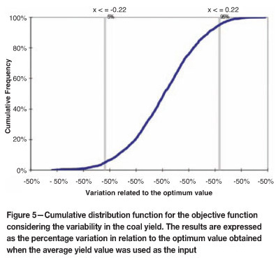
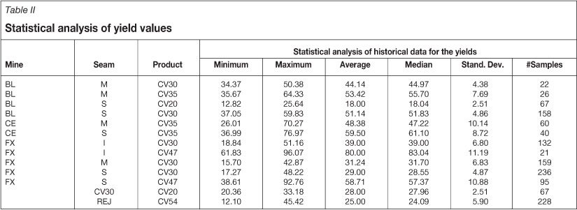
To illustrate the risk-analysis methodology, one of the optimized scenarios was chosen and the yield of different washed coals from different coal seams was considered as the parameter of stochastic behavior. The probability distributions of the yields were constructed using a historical series of results corresponding to the previous 12 months. The statistical summary for these variables is presented in Table II.

Two thousand draws from these probability distributions were retrieved and used to calculate the OF.

The variability obtained in the OF and in the coal yield are presented in Figure 5, which shows the relative variation between the results of the OF generated based on the simulated parameters and the results obtained by the optimization process considering coal yield as a fixed parameter. Analysis of the results obtained shows that:

The distribution of the results has a low asymmetry. This indicates that, in practice, there is no tendency for over- or underestimation of the OF value in relation to the optimum value obtained when the average yield was used as the input > The results present a high variability, ranging from -42 per cent to +39 per cent in relation to the optimum value of the OF, and 90 per cent of the values are between -22 per cent and +22 per cent.

 

 

To quantify the influence of each stochastic parameter in the results of the OF, the coefficient of linear correlation was calculated for the simulated values with respect to each parameter, and, subsequently, the OF values were calculated. The results of these calculations are shown in Figure 6.

 

 

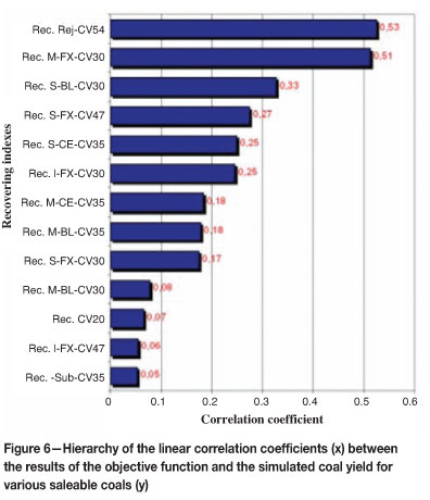
From Figure 6, it is noted that all the simulated parameters show a positive correlation with the results of the OF.

 

Discussion and conclusions

The results obtained fom mathematical modelling tools, optimization using LP, and risk analysis, suggest that financial gains can be obtained by using these techniques in mine planning. With these tools, the decisionmaker can evaluate a series of choices and hypotheses regarding the production process and thereafter conveniently propose structural changes in the process to generate a higher profit. Among the 10 scenarios analysed, the results of the optimization process indicate that the economic gains could increase by an average of 5.8 per cent, compared with the results obtained by the production strategies originally adopted by the company without any optimization process.

The results also show a large variability in the OF when the yields for the various coal products are used as stochastic inputs. This variability in the input is probably overestimated due to the use of historical data in the simulation process. The historical data used corresponds to a period of 12 months, during which mining occurred in different locations within the deposit. This fact can lead to significant variations in the product quality and yield. Hence, geostatistical simulation should be used to build coal-yield models and, after these simulations of the models are completed, the results obtained should be used to feed the yield values into the optimization process.

The use of a representative mathematical model for the production process generates other benefits, in addition to the tangible gains described previously. It allows a comprehensive understanding, transparency, and interaction of the production process, helping to quickly determine the influence of various factors on the response by different parameters related to this process. Consequently, the model can be used not only for the optimization of the current production process, but also to test alternatives such as the evaluation of new mine areas or the commercialization of other products. The correlation coefficient relating each stochastic parameter and the answers obtained by the OF can be used to rank the parameters that generate the greatest impact on the final value of this function. After the definition of the most relevant parameters, their behaviour can be more closely followed, and whenever possible, be directed toward values that improve the result of the OF.

The use of simulation techniques provides the opportunity to quantify the impact that the stochastic parameters produce in the optimum response. The stochastic approach enlarges the range of information available to the decisionmaker, allowing him or her to evaluate the risk of a given result, instead of depending on a single deterministic value of the OF.

 

References

1. Prado, D.S. Programajao Linear. Belo Horizonte, MG, Desenvolvimento Gerencial, 1999.         [ Links ]

2. Ravindran, A., Philips, D.T. and Solberg, J.J. Operations Research Principles and Practice. 2nd edn. John Wiley & Sons, New York, 1987.         [ Links ]

3. Loesch, C. and Hein, N. Pesquisa Operacional. FURB, Blumenau, 1999.         [ Links ]

4. Montevevechi, J.A.B. Pesquisa operacional (Programação linear). MSc. thesis, Escola Federal de Engenharia de Itajubá, 2000.         [ Links ]

5. Goldbarg, M.C. Otimização combinatória e programação linear: modelos e algoritmos. Rio de Janeiro, Campus, 2000.         [ Links ]

6. Dantzig, G.B. Linear Programming and Extensions. Princeton University Press, New Jersey, 1963.         [ Links ]

7. Fogliatto, F. Pesquisa operacional I - Modelos determinísticos. MSc.thesis, Universidade Federal do Rio Grande do Sul, Porto Alegre, 2004.         [ Links ]

8. BAZARAA, J. Linear Programming and Network Flows. 4th edn. Hoboken, New Jersey, John Wiley & Sons, 1999.         [ Links ]

9. Bronson, R. Pesquisa Operacional. Sao Paulo. MacGraw-Hill, 1985.         [ Links ]

10. Motta, R.R. Análise de investimentos - Tomada de decisão em projetos industriais. Sao Paulo, Atlas, 2002.         [ Links ]

11. Menner, W.A. Introduction to modeling and simulation. JohnsHopkins APL Technical Digest, vol. 16, no. 1, 1995.         [ Links ]

12 Freitas, P.J. Introdução à Modelagem e Simulação de Sistemas. Visual Books, Florianópolis, 2001.         [ Links ]

13. Schriber, T.J. Simulation using GPSS. New York, Wiley, 1974.         [ Links ]

14. Pegden, C.D., Shannon, R.E., and Sadowski, R.P. Introduction to simulation using SIMAN. New York, McGraw-Hill, 1990.         [ Links ]

15. Banks, J. and Carson, J.S. Discrete-event System Simulation. Prentice Hall College Div, New Jersey, 1984.         [ Links ]

16. Hartman, H.L. SME Mining Engineering Handbook., SME, Littleton Colorado, ,1992.         [ Links ]

17. Carvalho, J.A. Jr. Abordagem probabilistica em um modelo de programação linear aplicado ao planejamento mineiro. MSc. Thesis, Universidade Federal do Rio Grande do Sul, 2006.         [ Links ]

18. Lindo Systems Inc. Premier optimization modeling tools. http://www.lindo.com Accessed Jan. 2005.         [ Links ]

19. Bratley, P.,Fox, B.L., and Schrage, L.E. A Guide to Simulation. Springer-Verlag, New York, 1987.         [ Links ]

 

 

Paper received Aug. 2010
Revised paper received Dec. 2011