JOURNAL PAPER

 

Integrated short- and medium-term underground mine production scheduling

 

 

M. Nehring^I; E. Topal^II; M. Kizil^III; P. Knights^IV

^ISchool of Mechanical and Mining Engineering, The University of Queensland, St Lucia, QLD, Australia
^IIWestern Australia School of Mines, Curtin University of Technology, Kalgoorlie
^IIITeaching and Learning School of Mechanical and Mining Engineering, The University of Queensland, St Lucia, QLD, Australia
^IVMining Engineering School of Mechanical and Mining Engineering, The University of Queensland St Lucia, QLD, Australia

 

 

---

SYNOPSIS

The development of short- and medium-term mine production schedules in isolation from each other has meant that only a local optimum can be achieved when each scheduling phase is carried out. The globally optimal solution, however, can be achieved when integrating scheduling phases and accounting for the interaction between short-term and medium-term activities simultaneously. This paper addresses the task of integrating short- and medium-term production plans by combining the short-term objective of minimizing deviation from targeted mill feed grade with the medium-term objective of maximizing net present value (NPV) into a single mathematical optimization model. A conceptual sublevel stoping operation comprising 30 stopes is used for trialling segregated and integrated scheduling approaches. Segregated medium- and short-term scheduling using separate models achieved an NPV of $42 654 456. The final scheduling approach involved integrating the two scheduling horizons using the newly-developed globally optimal integrated production scheduling model to achieve an NPV of $42 823 657 with smoother mill feed grade. The larger the stope data set, the larger the difference between the two scheduling approaches is likely to be. At the very least, an integrated approach ensures feasibility across the two scheduling horizons, which cannot always be assumed when using a segregated approach.

Keywords: production scheduling, optimization, mixed integer programming, integrated scheduling, mine planning.

---

 

 

Introduction

The traditional mine production scheduling approach is to perform short- and medium-term scheduling as two separate phases, whereby the solution to one phase forms the starting point from which to carry out the next phase. The process will start with the establishment of a medium-term schedule that will span anywhere from the next two or three years of production through to the life of mine at monthly, quarterly, or even yearly intervals. The objective will be to maximize the Net Present Value (NPV) of the operation while maintaining all sequencing as well as tonnage and grade constraints. In open-pit mining this will generally result in a schedule that delays waste removal, while in underground mining a schedule that delays nonessential development will be preferred.

The next phase of the scheduling process will involve the establishment of a short-term schedule with the purpose of executing the long/medium-term scheduling results. At this stage more emphasis is placed on meeting production targets and achieving consistent production rates within the constraints of the operation. The value derived through the minimization of deviation from production targets may not be as visible from a purely mining operational perspective. However, from a processing plant viewpoint it is essential that consistent ore tonnages at consistent grades and quality are feed to the plant in order to maintain a stable and balanced operating environment. Any significant and abrupt changes are likely to initially disrupt this sensitive balance before altering the process to adjust to the changed feed supply. As such, value improvements (or maintaining the highest value) from a short-term perspective are achieved by ensuring a consistent feed.

The establishment of short- and medium-term mine production schedules in isolation from each other has meant that only a local optimum can be achieved when each scheduling phase is carried out. The globally optimal solution can be achieved only when integrating scheduling phases and accounting for the interaction between short-term and medium-term events simultaneously. As such, this paper presents an integrated mathematical scheduling model for use in sublevel stoping operations that accounts for the objectives of both scheduling horizons. A case study is presented that compares the results of a stope data set scheduled via separate medium- and short-term models and then by the integrated model.

 

Background

The use of operations research techniques is widely recognised for effectively modelling and solving complex problems. Mathematical programming, including those technique extensively described by Hillier and Lieberman (2001), tends to be particularly useful for application to large industrial problems. In the mining industry, processes amenable to optimization procedures are well documented by Alford (1995). In the underground environment the three core areas highly conducive to optimizations processes are stope boundary definition, decline and infrastructure layout, and production scheduling.

The latest advancements in relation to stope boundary definition and decline and infrastructure layout can be found in publications by, Sens (2008), Ataee-Pour (2005), and Alford (1995); and Brazil and Grossman (2008), Alford, et al. (2007), and Brazil and Thomas (2004) respectively. A number of authors have also made significant advances in both short- and medium/long-term mine production scheduling optimization.

A 23 percent increase in before- tax NPV from $273 million to $337 million was achieved by Trout (1995) with the development of a mixed integer programming production schedule (MIPPS) over a three-year period for 55 stopes in the 1100 orebody at Mount Isa, which uses the sublevel stoping method. Production was modelled according to four separate phases, with each represented by a corresponding binary and integer variable. The solution was obtained prior to proof of optimality after 1.6 hours on a powerful machine at the time. However, the schedule was not implemented and is open to a number of further improvements.

In ensuring geotechnical stability is maintained, Nehring and Topal (2007) successfully trialled a new MIP constraint formulation that limits fillmass exposure to a single side while limiting simultaneous stope exposure to no more than two sides for sublevel stoping operations. Following on from this, Little et al. (2008) achieved an 80 percent reduction in the number of variables, which in turn results in a 92 percent reduction in solution time for a small conceptual stoping operation by utilizing the natural progression of activity phases as stopes move through production.

An improved deviation from targeted production to just 6 percent via the new MIP model against 10-20 percent from manual scheduling was achieved by Topal (2003) when solving the problem of scheduling production of three products from two ore types at the Kiruna Mine. The use of 'machine placements', representing loader capacities containing a number of production blocks with an associated ore quantity of a certain quality in each time period, significantly increased efficiency by reducing the number of variables. In combination with the implementation of early and late start algorithms a solution time was achieved in under 100 seconds (Topal, 2008). The model was ultimately implemented into Kirunas' mainstream scheduling process.

The uncertainty surrounding equipment failure, geotechnical issues, and individual operator ability tends to make short-term production scheduling far more dynamic. Frequent re-running of the short-term scheduling model is often required in order to provide reassignments when necessary. Few items in the literature deal with the underground mine environment on a short-term basis. However, in open-pit mining, real-time machine allocation to cater for these dynamic circumstances has traditionally been handled by fleet management and dispatch systems.

Productivity improvements of between 7 percent and 20 percent have been reported in open literature at thirteen out of more than thirty open-pit mining operations after installation of Modular Mining Systems' DISPATCH system (White et al., 1993). The system itself comprises of three subsystems. Using raw mine topology of locations, elevations and roads, and distance data a best path (BP) algorithm generates the shortest path between all pairs of locations in the mine road network. Taking travel time and optimal routing data as well as pit configuration, available trucks and shovels, blending requirements and machine priority data from the BP, a linear programming (LP) subsystem model is then used to generate optimal path flow rates in tons per hour to minimize haulage requirements. Given a list of trucks needing an assignment and current travel times and distances a dynamic programming (DP) subsystem model finally provides assignments for each truck in real time.

LINDO software was used to solve a problem requiring the production of 80 000 t of ore and waste daily over three production shifts from the Sarcheshmeh open-pit copper mine in Iran (Osanloo and Saidy, 1999). A simple semi-dispatch system using linear programming with an objective of minimizing the total number of trucks required to meet production targets showed daily production could be achieved with just thirty, 120 t capacity trucks as opposed to the thirty-seven, 120 t capacity trucks originally planned. Variables in this case relate to the number of trucks assigned to each individual haulage path.

Development, testing, and validation of an algorithm to optimize shovel extraction sequences with the objective of minimizing ore tonnage deviation as well as minimizing grade deviation from predefined targets was successfully carried out on a hypothetical ore deposit over a seven-day 'rolling horizon' period at daily intervals, with reserves and shovel performance updated after each run (Knights and Li, 2006). The authors noted that mining blocks in a single period were sometimes not connected, thus requiring additional constraints to maintain equipment movement and relocations within a single period to an appropriate distance.

An enumeration algorithm based on dynamic programming for solving the fleet management problem in underground mines is proposed by Beaulieu and Ganache (2004). From an initial starting position for each machine, the objective is to find the best route and schedule for each machine such that their destination is reached in the shortest possible time. The solution approach is tested on 60 instances on three networks comprising of 20 instances per network with four machines in operation in each instance. The authors go into extensive detail about routing and displacement of machines throughout the network of underground drives and haul-routes in a concerted attempt to remain in a conflict-free state. Reality remains that the underground mine environment is very rigid, and in most cases there is only a single route a machine can feasibly take in the working of an ore-movement. Unlike open-pit dispatching, instances where multiple production machines are simultaneously operating on the same route are generally avoided, thus providing little justification for such a stringent focus on routing.

An underground active dispatch model (UADM) based on linear and goal programming is developed by Tsomondo (1999) to optimally allocate machines at the start of a shift based on static operating conditions. The active program allocates a machine to a single trip, after which it is free to request another job. A total of six dispatching policies are implemented into the model, with each able to be interchanged at will. These include: shortest travel time, earliest expected service time, minimum server-client slack time, maximum product quality, maximum quality with minimum slack time, and critical worksite ratio. While not all policies may be applicable in practise, the author compares the productivity of each policy as LHD fleet size is increased, concluding that each policy has a unique optimal fleet size for a given mine layout.

 

Model formulation

The model utilizes mixed integer programming (MIP) to model the integrated short- and medium-term mine production scheduling problem. Apart from dealing with the extraction of each stope and its subsequent ore movement, all external development, internal development, and production drilling and backfilling activities have also been incorporated into the model to provide a comprehensive integrated scheduling tool. All extraction-related items for both the short- and medium-term phases are presented in full, along with the formulations and constraints that tie together both scheduling horizons.

Subscript notation

The model is defined in general terms using the following subscript notation

t medium-term schedule time period: t = 1, 2, 3.... T

d medium-term external development identification: d = 1, 2, 3.... D

s medium-term stope identification: s = 1, 2, 3.... S

f existing fillmass identification

m short-term machine identification: m = 1, 2, 3.... M

m' refers only to LHDs

m" refers only to trucks

o short-term ore movement identification: o = 1,2,3.,

O

o' refers only to primary ore-movements

o" refers only to flow on secondary ore movements

θ refers to each ore movement within S_o not able to simultaneously share the same machine with ore movement o

short-term scheduling interval period: i = 1,2,3..., I i.

Sets

Several sets are defined which aid in the formulation of constraints.

α^d set of eligible medium-term time periods in which external development item d can be in production

αt set of eligible external development items d which can be in production in medium-term time period t

β_s set of eligible medium-term time periods in which stope s can be in production

βt set of eligible stopes that can be in production in medium-term time period t

dbdd set of external development items that can be accessed only after the completion of external development item d

dbmd set of stopes that can commence production only after the completion of external development item d

adjs set of all stopes that are adjacent to and share a boundary with stope s

badjf set of all stopes that are adjacent to and share a boundary with each each existing fillmass f

tpbt set of time periods that include all periods up to the current period t

Po set of intervals in which ore movement o is available for production

No set of intervals in which ore movement o is unavailable for production

Io" set of primary ore movements o' that flow on into each secondary ore movement o"

Qi set of intervals that includes all intervals up to and including the current interval

Ro' the primary ore movement o'⁺¹ that must proceed primary ore movement o' in order to maintain the natural stope extraction sequence

So set of ore movements è that are not conducive to simultaneously sharing the same machine with ore movement o

L_m set of ore movements that are not conducive to haulage by machine type (e.g. trucks are used when hauls are over 3000 m in length, LHDs are used for everything else)

Z_t set of short-term intervals i corresponding to each medium-term period t

so_s set of ore movements o associated with the production of each stope s.

Parameters

These parameter items represent the numeric inputs and conditions.

n_t present value discount factor for time period t

dcf_d undiscounted cash flow ($) from each external development item d

cf_s undiscounted cash flow ($) from each stope s

pena penalty factor ($) applied to each tonnage of deviation above target

penb penalty factor ($) applied to each tonnage of deviation below target

W short-term penalty weighting factor

de_d earliest start time for external development item d

dl_d latest start time for external development item d

e_s earliest start time for stope s

l_s latest start time for stope s

dr_d extraction reserve (t) for each external development item d

r_s extraction reserve (t) for each stope s.

sc_t shaft/LHD/truck fleet movement capacity (t) for each time period t

dgld difference between targeted lower ore feed head grade and the grade of each external development item d

gls difference between targeted lower ore feed head grade and the grade of each stope s

dgud difference between targeted upper ore feed head grade and the grade of each external development item d

gu_s difference between targeted upper ore feed head grade and the grade of each stope s

edm_d length (m) of each external development item d

idm_s length (m) of internal development required for each stope s

dc_t development fleet capacity (m) for each time period t drl_s length (m) of production drilling required for each stope s

drc_t drilling fleet capacity (m) for each time period t

bk_s backfill (t) required for each stope s

bkc_t backfill availability (t) for each time period t

res_o' ore reserve contained within primary ore-movement o'

gra_O´ difference between targeted short-term mill feed grade and actual ore grade of primary ore-movement o'

msc_t ore tonnage capacity of haulage shaft in interval i

mt_m task limit (number of assignments) for machine m

nml_O number of LHDs able to work simultaneously on ore movement o

nmt_o number of Trucks able to work simultaneously on ore movement o

mc_mi capacity of machine m in interval ii. Expressed in ton-metres per interval (bucket capacity (t) multiplied by average working speed (m/h) multiplied by operating time (h) per interval)

dst_O return length (metres) of ore movement o

ml_m lowest feasible machine m movement (t)

M large number, M = 10 000 000

sop_so link between the ore movements of each stope s and the periods each ore movement is expected to be available once production on the stope is initiated. If available = 1, if not = 0.

Decision variables

A total of three linear and two binary variables were required to reflect operating conditions and ultimately perform the scheduling task.

Vd_t 1 if production from development item d is scheduled for time period t

0 otherwise.

W_st 1 if production from stope s is scheduled for time period t 0 otherwise.

X_moi ore tonnes extracted by machine m from ore movement o in interval i.

Y_moi 1 if extraction by machine m of ore movement o takes place in interval i 0 otherwise.

a_i metal tons produced above the predefined target in interval i.

b_i metal tons produced below the predefined target in interval i.

Objective function

The objective function seeks to maximize the NPV of all activities under consideration by determining the optimal schedule within which to progress each stope through production. A weighted cash penalty is applied to each ton of metal produced above and below the predefined target for each short-term interval.

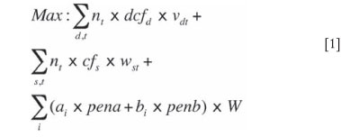
In this case the penalty factors are negative values. It should also be noted that taxation and depreciation are not included in this formulation, although they should be incorporated if necessary.

Constraints

The globally optimal integrated production scheduling model comprises numerous constraints that reflect the practical limitations imposed by the sublevel stoping method over both the medium and short-term scheduling horizons. These constraints can be classified according to the limitations they impose on resources, sequencing, or timing.

Medium-term resource constraints

The following formulations display the mathematical resource constraints that are applicable across the medium-term horizon.

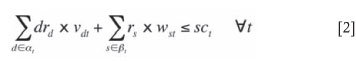
Shaft/machine fleet ore capacity constraint

Lower mill feed grade limit constraint

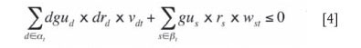
Upper mill feed grade limit constraint

External and internal development activity constraint

Production drilling activity constraint

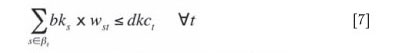
Backfill availability constraint

Non-negativity and integer value constraint

Constraint [2] limits production of all development and stope extraction ore from exceeding the shaft/LHD/truck fleet capacity in any medium-term time period. Constraint [3] restricts the combined mill feed grade of all development and stoping ore from exceeding a lower grade limit in any medium-term time period. Constraint [4] restricts the combined mill feed grade of all development and stoping ore from exceeding an upper grade limit in any medium-term time period. All external and internal development activities are restricted to an operations' development fleet capacity in each medium-term time period by constraint [5]. Constraint [6] ensures that production drilling in any medium-term time period is with the drilling fleet capacity limit. Backfill availability in each medium-term time period is enforced by constraint [7]. Constraint [8] enforces non-negativity and integer values of the appropriate variables.

Medium-term sequencing constraints

The following formulations display the mathematical sequencing constraints that are applicable across the medium-term horizon.

External development precedence sequencing constraint

Non-concurrent external development sequencing constraint

External development to stope production precedence constraint

Non-concurrent external development to stoping sequencing constraint

Stope production precedence sequencing constraint

Non-concurrent stope sequencing constraint

Stope adjacency constraint

Fillmass adjacency constraint

Existing fillmass adjacency constraint

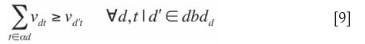
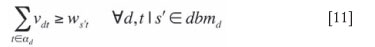
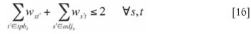
Constraints [9] and [10] ensure that the sequencing between external development items is maintained by allowing those items that follow on from other items to commence only after the completion of their predecessor. Constraints [11] and [12] enforce appropriate sequencing between external development items and stope production by ensuring stope production commences only after the completion of all necessary external development. All preceding and future production sequencing, between stopes is also enforced by constraints [13] and [14]. Constraint [15] ensures that simultaneous production between stopes that share a common boundary does not occur. Constraint [16] ensures geotechnical stability of each stope by limiting simultaneous adjacent production to two common boundaries before the stope under consideration has itself commenced production, and to a single adjacent side once having completed production to become a fillmass. Constraint [17] ensures fillmass stability of all existing fillmasses by limiting exposure to a single common boundary in each medium-term time period.

Medium-term timing constraints

The following formulations display the mathematical timing constraints that are applicable across the medium-term horizon.

May develop constraint

Must develop constraint

May mine constraint

Must mine constraint

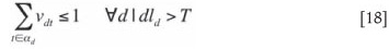
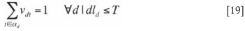
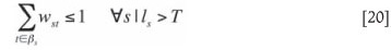
Constraint [18] ensures that the commencement of external development items is initiated no more than once during the medium-term scheduling horizon if their late start date occurs beyond the scheduling horizon. Constraint [19] requires that external development items commence at some point during the medium-term scheduling horizon if their late start date falls within the medium-term scheduling horizon. Constraint [20] ensures that commencement of stope production is initiated no more than once during the medium-term scheduling horizon if the late start date occurs beyond the scheduling horizon. Constraint [21] requires stope production commences at some point during the medium-term scheduling horizon if the late start date falls within the medium-term scheduling horizon.

Short-term resource constraints

The following formulations display the mathematical resource constraints that are applicable across the short-term horizon.

Target mill feed grade balancing constraint

movement ore reserve extract constraint

Short-term interval haulage shaft capacity

Individual machine capacity constraint

Orepass throughput balance constraint

Minimum feasible movement constraint

Short-term variable linking constraint

Machine type to ore movement constraint

Non-negativity and integer value constraints

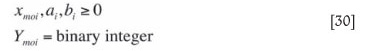
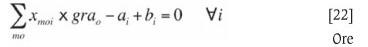
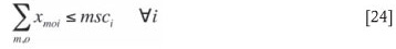
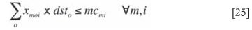
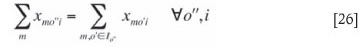
Constraint [22] ensures that metal tons for the respective target mill feed grade produced across all machines from primary ore movements in each short-term interval balances with the metal tonnage excess ai or shortfall bi deviation for the respective ore tonnage being processed. Constraint [23] ensures that ore production from each primary ore movement does not exceed its reserve. Primary ore movement ore production in any short-term interval cannot exceed the haulage shaft capacity as enforced by constraint [24]. Constraint [25] ensures that the ore tonnage moved by each production machine in each short-term interval cannot exceed the individual capacities of the machines. Constraint [26] ensures that throughput across each secondary ore movement balances with ore from inflow primary ore movements in each interval. Constraint [27] ensures that a minimum tonnage must be moved (in this case 10 t) for it to be feasible for a machine to be assigned to an ore movement. This constraint also ensures that if xmoi = 0 -^Y_moi- = 0. Constraint [28] ensures that if xmoi is utilized, Ymoi must equal 1. Constraint [29] ensures that LHDs are not assigned to truck routes and trucks are not assigned to LHD routes. Finally, constraints [30] enforce non-negativity and integer values of the appropriate variables.

Short-term sequencing constraints

The following formulations display the mathematical sequencing constraints that are applicable across the short-term horizon.

Machine task limit constraint

Simultaneously operating LHD constraint

Simultaneously operating truck constraint

Ore-movement sequencing constraint

Simultaneous LHD share constraint

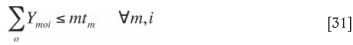
In order to limit the amount of productive time wasted by machines tramming between jobs, a machine will generally be assigned to no more than a predetermined number of ore movements during any given short-term interval, as enforced by constraint [31]. Constraints [32] and [33] ensure that the number of machines (LHDs m' and trucks m'' respectively) operating simultaneously on any given ore movement in any interval does not exceed the physical limitation of the ore movement itself. Constraint [34] ensures full reserve production from each primary ore movement before production from the proceeding primary ore movement can commence, thus maintaining the natural sequential transition into production from one ore movement to the next.

Constraint [35] ensures that all pairs of ore movements that are not located in close proximity to each other and therefore do not feed into the same ore-pass system are not able to simultaneously share the same machine.

Short-term timing constraint

The following formulation displays the mathematical timing constraint that is applicable across the short-term horizon. Ore-movement availability constraint

The production availability of ore movements and any short-term interruptions are able to be taken into account by constraint [36].

Medium/short-term integration constraint

The following formulation displays the mathematical integration constraint to ensure feasibility across both scheduling horizons.

Constraint [37] performs two crucial roles. It firstly ensures that if an ore movement is selected for production, its entire reserve is extracted during its production availability period. Secondly, it also provides the critical link between short- and medium-term variables by essentially forcing the simultaneous medium and short-term production scheduling of a stope and all its respective ore movements if it is selected to be part of the schedule.

 

Application of integrated model

For the purpose of comparing the integrated scheduling model against segregated medium and short-term scheduling results, a small conceptual operation utilizing the sublevel stoping method is used as a trial case study. This operation has little capacity for stockpiling and has its ore toll-treated at a nearby facility. In negotiating use of this facility, stringent mill feed grade parameters had to be maintained. As such, the agreement outlined that in addition to a standard treatment charge per ton of ore, each ton of copper production above target for the respective ore tonnage being processed in each interval attracts a penalty of $3000. Each ton of copper production below target for the respective ore tonnage being processed in each interval attracts a penalty of $3500.

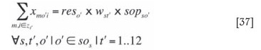
Stope production is represented by four phases, commencing with internal development followed by production drilling and ore extraction before backfilling takes place. As shown in Figure 1, the operation comprises a total of 30 stopes, three of which have already completed the entire production process to become a fully consolidated fillmass, one undergoing internal development, one in the production drilling phase, two in the ore extraction phase, and one undergoing backfilling, leaving the remaining 22 stopes available for the commencement of production with the internal development phase, subject to the completion of all necessary preceding external development activities.

 

 

In scheduling production from this operation all adjacency interactions for all stopes as well as existing and future fillmasses are enforced. During each month of production the operation's ore handling system, including the main haulage shaft, is restricted to 95 000 t at a combined blend of no less than 1.8 percent Cu and no greater than 2.6 percent Cu. The operation's medium-term schedule spans one and a half years at monthly intervals for a total of 18 months, whereby the objective is to maximize NPV at a discount rate of 10 percent per annum. In addition, the first twelve months, production will undergo short-term scheduling, with each month being divided into four equal intervals for a total of 48 short-term intervals over which the objective is to minimize deviation from a targeted mill feed grade of 2.20 percent Cu for an upper ore limit of 25 000 t.

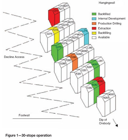
The remaining 22 stopes contain a combined reserve of 4.24 Mt of ore grading 2.20 percent Cu for 92 160 t of copper metal. Once extracted from drawpoints via LHD, ore is channelled to an underground crusher station through a series of ore-passes before being hoisted to the surface via the haulage shaft, as illustrated by the ore flow overview diagram in Figure 2, which also shows each stope allocated to its respective orepass.

 

 

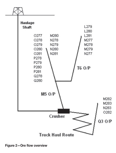
As shown in Figure 2, ore from the majority of stopes is tipped into the M5 orepass, which feeds directly to the crusher. Ore from the T6 orepass, which also services a number of stopes in the upper part of the orebody, requires rehandling before also being tipped into the M5 orepass at an LHD transfer level. Depth extensions to the orebody have resulted in mine expansion activities below the current crushing horizon. As a result, ore from stopes M282, M283, N283, and O283 is tipped into the Q3 orepass, which channels ore to a central truck loading facility from where it is hauled up the haul route to the crusher. Table I presents the complete route (including primary and secondary ore movements) that ore from each stope must take in order to reach the crusher, and the respective return-trip LHD and truck cycle distances associated with each primary and secondary ore movement.

 

 

In addition to all primary and secondary ore movements, a total of 21 external development items associated with various stopes are also required to be scheduled, together with all relevant precedence information as outlined in Table II.

 

 

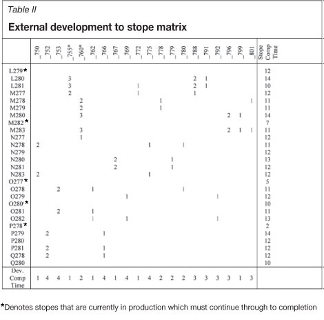
The numbering system in this case defines which external development item need to be completed for each respective stope in descending order (the highest first, followed by the second highest, etc). To ensure continuity and a smooth transition from the current scheduling regime to the new one, all stopes and external development items that are currently active will be seen through to completion. Coloured numbers represent different activity streams that do not have any sequencing inactions with other streams for the respective stope. Also presented in Table II are the expected completion times (months) once commencement has been initiated for each stope and external development activity. To form the basis for medium-term scheduling, an ore tonnage (t) and grade (percent Cu) distribution can be generated for each stope over each monthly period once commencement is initiated. The results are shown in Table III for a selected number of stopes.

 

 

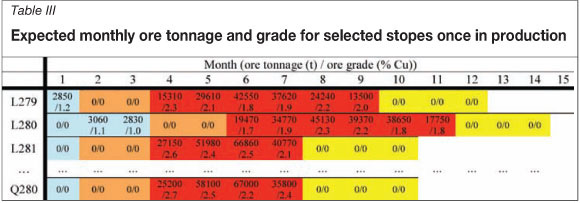
As shown in Table III, the production life of stope L279 spans across a 12-month period. An expected total of 2 850 t of internal development ore at 1.2 percent Cu in its first month once production is initiated is scheduled for processing. This is followed by a two-month period of production drilling, which then leads into a six-month ore extraction phase producing a total of 162 830 t at an average grade of 2.0 percent Cu. A similar table may also be established for those external development items that produce ore of high enough grade to be sent to the surface for processing. All development rates, production drilling rates, and backfill placement are also predefined for each stope and is limited to 200 meters, 18,000 m, and 160 000 t respectively across all stopes in each month.

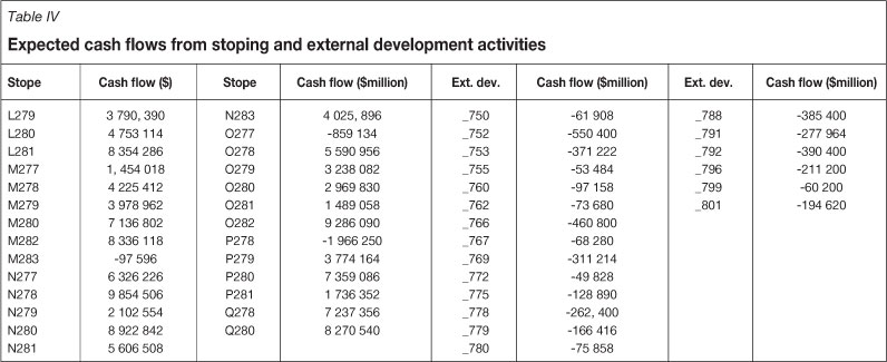
Using the production rates in Table III and expected development and production drilling rates as well as backfill tonnages associated with each stope, an expected cash flow associated with each activity (using predetermined copper prices, copper recoveries, fixed and variable cost of development and drilling per unit length, extraction costs per ton, as well as the cost of backfill) can be calculated. The expected cash flows for each stoping and external development activity are presented in Table IV.

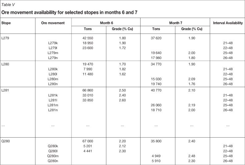
For the purpose of short-term scheduling it becomes necessary to break down monthly production from each stope into smaller more definable blocks in order to more appropriately reflect the grade fluctuations that naturally occur during the course of production, and thus aid the short-term objective of minimizing deviation from the targeted mill feed grade. As a result of this, the tabulated medium-term production data for each stope in Table III is reworked further into its individual primary ore movement availability before being presented to the mathematical model for evaluation. This is an activity that should be carried out in any case by any operation seeking reliable grade controls even under a manual scheduling regime. Table V presents the production tonnages and grades, as well as the availabilities of selected primary ore movements, over their sixth and seventh months of production.

As shown, the expected 42 550 t at 1.80 percent Cu produced from stope L279 in its sixth month of production in reality comprises two individual primary ore movements, including 18 950 t at 1.90 percent Cu and 23 600 t at 1.72 percent Cu. Determination of all ore-movement availabilities has thus increased the initial 27-stope production data set into substantially more primary ore movements for consideration across the forty-eight intervals. Anticipating the timeframe that each ore movement within a stope for a particular operation will be available to a high level of accuracy is not an easy task. The further away a particular ore movement is from production the more difficult this becomes. This is therefore an activity that relies on the judgement of an experienced person.

In order for machine allocations to take place over each short-term interval, individual machine capacities must be known and placed to the model for evaluation. Table VI presents the main parameters that are multiplied together to achieve a capacity value suitable for input into the mathematical model. For shifts where a machine is taken out of service for maintenance or noncore activities, operating hours for that interval are adjusted accordingly.

The maximum number of tasks or ore movements that each LHD and truck can be assigned to during any given interval has been limited to four and two respectively. For any machine to be assigned to an ore movement, a minimum of 10 t must be moved.

Also important to consider in short-term scheduling and machine allocation is the number of simultaneously operating LHDs each ore movement is able to contain. In most cases the physical limitations and rigidness of the haul route itself is able to reasonably support only a single LHD operating at full speed and capacity during a given interval. Due to each interval in this case spanning just over seven days, a maximum of two loaders are able to operate simultaneously on each ore movement within each interval. Multiple trucks, however, are able to operate simultaneously along the designated haul route.

Each ore movement's ability to share an LHD unit with another ore movement in any given interval should also be considered. This is appropriate when ore movements are located in close proximity to each other with ore possibly being directed into the same ore pass, or where ore that requires rehandling is tipped into an ore pass and again moved from the base of the ore-pass by the same LHD. Due to the close proximity of all stopes in this operation, LHD sharing between all ore movements during each interval is allowed except for the LHD assigned to loading trucks at the base of the Q3 orepass, which must always be available as trucks cycle back and forth to the crusher.

 

Results

Construction of all models took place using A Mathematical Programming Language (AMPL), which was then solved using CPLEX 10.3 on a standard office computer. Having established all short- and medium-term scheduling parameters, a medium-term production schedule spanning 18 months using the medium-term mathematical production scheduling model with the objective of maximizing NPV was generated. The results of this are displayed in Figure 3.

 

 

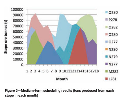
As shown, ore production across the 18 monthly periods fluctuates quite significantly. The resulting locally optimal medium-term schedule produced an NPV across the scheduling horizon of $46 274 056. Ore production commences with M282 and O277, followed closely by O280, which represents a continuation of those stopes already in production. A combination of production and sequencing constraints and external development activities required beforehand results in the best stope (N278), on a cash flow per month in production basis, being completely left out of the schedule. While the values (on a cash flow per month in production basis) of stopes such as N277, N279 and O282 are reasonably high, they are by no means the highest. While this is only a small operation, the complexities surrounding sequencing issues relating to void size and fillmass stability are very prominent. Having to manually evaluate each possible scheduling scenario would be very time-consuming. As such, a rapid evaluation of each scheduling scenario can be conducted only through a mathematical optimization model. As more stopes and time periods are added to the data set, the complexity of the problem increases exponentially.

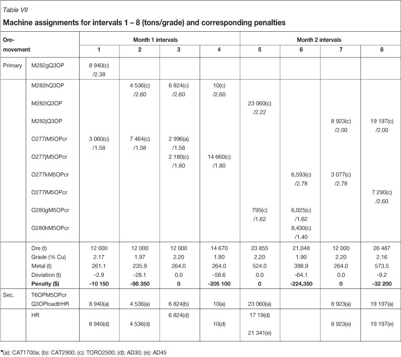
Following on from this, the first twelve months, production results can be taken for input into the short-term production scheduling and machine allocation process. The ore-movement production data in Table V for all stopes that are selected for production can therefore be presented to the short-term mathematical production scheduling model with the objective of minimizing deviation to the targeted mill feed grade of 2.20 percent Cu across all 48 short-term intervals. A $3 000 penalty for each ton of over-production and a $3 500 penalty for each ton of under-production for the respective ore tonnage being processed are applied. Table VII shows machines assigned to ore-movements and the respective tonnage to be produced from each assignment, together with the corresponding penalties applicable to each of the first 8 intervals.

Across all forty-eight intervals a total production of 876 460 ton of production ore at an average grade of 2.17 percent Cu containing 19 026 t of copper is achieved. With a target mill feed grade of 2.20 percent Cu, ten of the 48 short-term intervals exceeded this target resulting in the production of an additional 423 t of copper metal for the ore tonnage being processed. A further 20 intervals fell short of targeted mill feed grade, resulting in shortfall production of 671.6 t of copper metal for the ore tonnage being processed with the remaining 18 intervals achieving the targeted grade. When taking into account the $3 000 and $3 500 penalties applied to all excess and shortfall production respectively, this results in a total applicable penalty of $3 619 600. When subtracting this amount from the NPV contribution of the medium-term schedule, this results in a final NPV of $42 654 456 ($46 274 056-$3 619,600).

The same data set under the same parameters is presented to the integrated mathematical scheduling model. Table VIII compares the NPVs and corresponding month of commencement of each stope between the segregated and integrated scheduling approaches respectively.

 

 

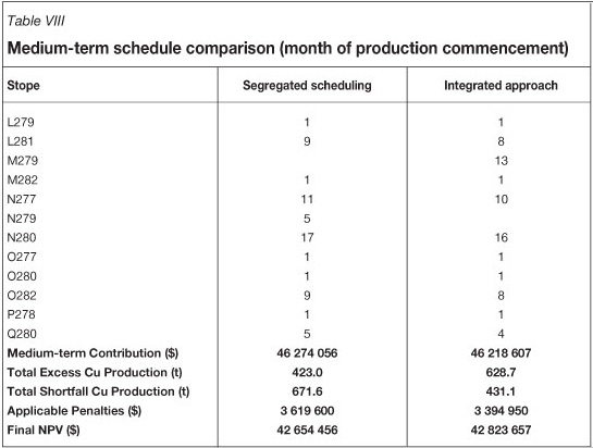
It is apparent that some significant changes in the schedule have taken place, with stope N279, which commenced production in the fifth month under the segregated approach having been completely left out under the integrated approach. This, however, provides the opportunity for stope M279 to enter the schedule in month 13. In addition to this, stopes L281, N277, N280, O282, and Q280 all commence production a month earlier. This change results in the medium-term schedules' contribution to NPV of $46 218 607. In comparison to the segregated locally optimal result this represents a decrease of $55 449 in value.

The resulting impact of altering the medium-term schedule is an overall increase of 205.7 t to 628.7 t in the copper tonnage produced as a result of exceeding target mill feed grade across the 48 short-term intervals. The overall shortfall in copper metal production due to shortfalls in the target mill feed grade decreases by 240.5 t to 431.1 t over the segregated short-term schedule. This thus has the overall net effect of reducing total applicable penalties from $3 619 600 to $3 394 950, representing a decrease of $224 650.

It is evident that the integrated model found that it is actually best to lower the NPV contribution made by the medium-term in favour of reduced short-term penalties, resulting in the optimal final NPV. Taking into account the overall value of both the medium-term schedule and the corresponding short-term schedule, it is evident that while a feasible result may be obtained through separate optimization processes, only an integrated optimization tool can guarantee a globally optimal scheduling solution. By fully considering the interactions between short- and medium-term scheduling, the integrated scheduling model was able to improve final NPV by $169 201 to $42 823 657 over the result that would otherwise have been obtained by using the traditional approach of obtaining a solution to the medium-term problem before then solving the short-term problem.

This represents a 0.4 percent increase in NPV over the segregated optimal schedule. As the size of the data set increases, it would be reasonable to expect greater gains in value. In any case, this represents additional value that may not have otherwise been achieved. This integrated scheduling approach can thus provide scheduling engineers with a powerful tool to aid the decisionmaking process. While it can be argued that the difference in final NPV between the locally optimal segregated and globally optimal integrated schedules is too small to warrant its further use, it must be recognised that there is one other very significant benefit of integrated scheduling. Due to the extensive usage of bulk resource capacities in medium-term scheduling (eg. LHD/truck fleet capacities), an activity which may be feasible in a particular month in the medium-term is not actually feasible in a corresponding short-term interval once more detail is added and machine allocation takes place. Therefore, even if the results of a globally optimal integrated schedule do not differ to that of the locally optimal segregated schedule, use of the integrated process ensures that an activity in one horizon must also occur in the corresponding horizon. This cross-referencing process thus ensures feasibility between the two scheduling horizons. This would otherwise be identified only during the short-term scheduling process when the mathematical model generates a run error due to an infeasi-bility issue, which would otherwise take a significant amount of time to manually identify and correct.

 

Conclusion

This paper has demonstrated that an integrated scheduling tool can provide a powerful means for obtaining the globally optimal scheduling result by taking into consideration all interactions that occur across the medium and short-terms.

Since a fixed price is applied to each ton of excess and shortfall metal deviation, at an operational level, the point at which to actually switch to the alternative plan is simple as this will depend solely on the highest NPV.

In this case, the application of the optimal integrated scheduling approach to a small operation having its ore toll-treated and thus being charged a $3, 000 and $3 500 penalty for each ton of excess and shortfall metal deviation to targeted mill feed grade for the respective ore tonnage being processed, increases final NPV by 0.4 percent over the segregated approach. While a relatively small increase, this represents additional value being extracted from a process that is already currently recognized as being optimal, as both medium and short-term scheduling phases are solved using a rigorous mathematical programming model.

At the very least, an integrated approach ensures that whatever schedule is selected in the medium-term is actually feasible from a short-term perspective also. Due to the use of fleet capacities and other bulk grouped equivalent capacities, it can be common for the medium-term schedule to be infeasible over the short-term due to a certain capacity constraint being exceeded, which can not actually be presented in the level of detail in the medium-term that would otherwise be required.

 

Future developments

The use of a penalty system applied to each ton of metal deviation to target for the respective ore tonnage being processed as used in this paper lends itself to a number of alternative short-term scheduling strategies that can be incorporated into the integrated model, depending on the scheduling and operational objective. In this case, shortfall deviation is to be avoided more so than excess deviation, thus a greater weighting is attributed to shortfall deviation. It may also be in the best interest of an operation to place a greater emphasis on achieving target production for near-term intervals. This can be achieved by assigning intervals a greater weighting the closer they are.

Placing an emphasis on production smoothing in order to avoid spikes in deviation from one interval to the next may also provide benefits to an operation. Assigning penalties that increase with an increase in deviation may be one way of addressing this issue.

 

REFERENCES

ALFORD, C. 1995. Optimization in underground mine design. Conference Proceedings of the 25th International APCOM Symposium. Australasian Institute of Mining and Metallurgy, Melbourne. pp. 213-218.         [ Links ]

ALFORD, C., Brazil, M., et al. (2007). Optimization in underground mining. Handbook of Operations Research in Natural Resources. New York, Springer. pp. 561-577.         [ Links ]

ATAEE-POUR, M. 2005. A critical survey of existing stope layout optimization techniques. Journal of Mining Science, vol. 41, no. 5. pp. 447-466.         [ Links ]

BEAULIEU, M. and GAMACHE, M. 2004. An enumeration algorithm for solving the fleet management problem in underground mines. Computers & Operations Research. pp. 1606-1624.         [ Links ]

BRAZIL, M. and P. GROSSMAN, A. 2008. Access layout optimization for underground mines, Australian Mining Technology Conference, Twin Waters. The Australasian Institute of Mining and Metallurgy, Melborne.         [ Links ]

BRAZIL, M. and THOMAS, D.A. 2004. Network optimization for the design of underground mines. Networks, vol. 49, no. 1. pp. 40-50.         [ Links ]

HILLIER, F.S. and LIEBERMAN, G.J. 2001. Introduction to Operations Research. Boston, Mass, McGraw Hill.         [ Links ]

KNIGHTS, P.F. and LI, S. 2006. Short-term sequence optimization - problem definition and initial solution. Proceeding of the Australian Mining Technology Conference (CRC Mining). The Australasian Institute of Mining and Metallurgy, Melbourne. pp. 385-394.         [ Links ]

LITTLE, J., NEHRING, M., and Topal, E., 2008. A new mixed-integer programming model for mine production scheduling optimization in sublevel stope mining. Proceedings of the Australian Mining Technology Conference (CRC Mining), Melbourne. The Australasian Institute of Mining and Metallurgy. pp. 157-172.         [ Links ]

NEHRING, M. and TOPAL, E. 2007. Production schedule optimization in underground hard rock mining using mixed integer programming. Proceedings - Project Evaluation. The Australasian Institute of Mining and Metallurgy, Melbourne. pp. 169-175.         [ Links ]

OSANLOO, M. and SAIDY, S.H. 1999. The possibility of using semi-dispatching systems in Sarcheshmeh copper mine of Iran. Computer Applications in the Minerals Industries, (Colorado School of Mines, Golden) pp. 243-252.         [ Links ]

SENS, J. 2005. Stope boundary optimization. B.Eng. thesis. The University of Queensland, Brisbane.         [ Links ]

TOPAL, E. 2003. Advanced underground mine scheduling using mixed integer programming. PhD thesis, Colorado School of Mines, Colorado.         [ Links ]

TOPAL, E. 2008. Early start and late start algorithms to improve the solution time for long term underground mine scheduling. Journal of the Southern African Institute of Mining and Metallurgy, vol. 108, no. 2. pp. 99-107.         [ Links ]

TROUT, L P. 1995, Underground mine production scheduling using mixed integer programming. Proceedings of the 25th International APCOM Symposium, Melbourne. The Australasian Institute of Mining and Metallurgy. pp. 395-400.         [ Links ]

TSOMONDO, C.M. 1999. A flexible underground mining system with active dispatching model - a solution for the next millennium. Computer Applications in the Minerals Industries, Golden, Colorado School of Mines. pp. 463-473.         [ Links ]

WHITE, J.W., OLSON, J.P., and VOHNOUT, S.I. 1993. On improving truck/shovel productivity in open pit mines, CIM Bulletin, September, 1993. pp. 43-49.         [ Links ]

 

 

Paper received Jan. 2011
revised paper received Nov. 2011