SPECIAL EDITION

 

Fitness landscape measures for analysing the topology of the feasible region of an optimisation problem

 

 

N.J. van der Westhuyzen^*; J.H. van Vuuren

Stellenbosch Unit for Operations Research in Engineering, Department of Industrial Engineering, Stellenbosch University, Stellenbosch, South Africa

 

 

---

ABSTRACT

Fitness landscape analysis has found numerous applications in industrial engineering, such as estimating optimisation problem complexity, predicting metaheuristic performance, and automating algorithm selection. In these applications, relationships between properties of the fitness landscape and metaheuristic algorithmic appropriateness are often analysed. The ability of a metaheuristic to traverse diverse areas of the feasible region is, however, typically overlooked when analysing algorithmic performance by invoking traditional measures of fitness landscape characteristics. In this paper, we propose three novel fitness landscape measures that are tailored to analyse the structure and degree of connectedness of the feasible region. These measures are related to the degree of neighbourhood feasibility, the size of the feasible region relative to that of the entire search space, and the tightness of the constraints. The significance of these measures is demonstrated in a suite of fitness-landscape analyses. When incorporated into a metaheuristic configuration machine-learning model, the measures yield accuracy improvements up to 6.4%.

---

OPSOMMING

Fiksheidslandskap-ontleding het talle bedryfsingenieurswese toepassings gevind, soos die afskatting van optimeringsprobleemkompleksiteit, die voorspelling van metaheuristiese prestasie en die outomatisering van algoritme-seleksie. In hierdie toepassings word verwantskappe tussen eienskappe van die fiksheidslandskap en metaheuristiese algoritmiese toepaslikheid dikwels ontleed. Die vermoë van 'n metaheuristiek om diverse gebiede van die toelaatbare gebied te deurkruis, word egter tipies oor die hoof gesien wanneer algoritmiese prestasie deur middel van tradisionele maatstawwe van fiksheidslandskapeienskappe ontleed word. In hierdie artikel stel ons drie nuwe fiksheidslandskapmaatstawwe voor wat aangepas is om die struktuur en graad van samehang van die toelaatbare gebied te ontleed. Hierdie maatreëls hou verband met die graad van buurpunt-toelaatbaarheid, die grootte van die toelaatbare gebied relatief tot dié van die hele soekruimte, en die strengheid van die beperkings. Die belangrikheid van hierdie maatreëls word in 'n reeks fiksheidslandskap-ontledings gedemonstreer. Wanneer die maatstawwe in 'n metaheuristiese konfigurasie-masjienleermodel opgeneem word, lewer hul akkuraatheidsverbeterings van tot 6.4%.

---

 

 

1. INTRODUCTION

The notion of a fitness landscape was first introduced in 1932 by Sewall Wright [1] in the context of genetic evolution, with follow-up work published 56 years later, in 1988 [2]. The abstract notion of a 'fitness' landscape, formed by placing neighbouring solutions of differing quality (or fitness) side by side, gave rise to the field of fitness landscape analysis (FLA). The field has since grown significantly in a variety of domains of the literature. A central area of focus in FLA has developed around gaining a better understanding of the factors that influence metaheuristic optimisation performance. This has become especially beneficial during the process of algorithm selection.

Many valuable contributions have been made to gaining unique empirical perspectives of the fitness landscape by evaluating a variety of FLA measures proposed in the literature. These measures are typically designed with a specific objective in mind, such as extracting crucial information about a particular fitness landscape feature or characteristic. Such a characterisation of the fitness landscape is typically achieved in a graphical and/or numerical fashion (such as a scalar representation of the degree of ruggedness of the fitness landscape).

It is well known that metaheuristics often fail to uncover local optima of sufficiently high quality, and leave practitioners with little to no information as to the reason for the failure. This forces practitioners to use trial-and-error procedures for metaheuristic configuration and hyper-parameter tuning, or even to pursue other metaheuristic designs that may seem intuitively better suited to the optimisation problem at hand [3], [4]. Collectively, the implementation of a variety of these measures may aid in gaining a conceptual understanding of problem complexity, and assist in identifying possible stumbling blocks that a metaheuristic may encounter during its search process.

In general, these FLA measures are capable of providing valuable perspectives on the nature and potential complexity of the problem under consideration, although they currently appear to exclude any consideration of solution feasibility - a vital consideration for the efficacy with which a metaheuristic can traverse the fitness landscapes. To the best of our knowledge, the only study in which solution feasibility and infeasibility were incorporated into FLA is that of violation landscapes proposed by Malan et al. [5] in 2015. Evaluation of this measure, however, involves the use of a so-called violation function (quantifying the extent to which a candidate solution violates the problem constraints) in the definition of an entirely new landscape rather than characterising the original landscape under consideration.

We consider fitness landscape feasibility structures as a vital part of the pursuit of a better understanding of good or poor metaheuristic search performance, because different metaheuristics (and metaheuristic configurations) handle solution infeasibility differently, resulting in different modes for traversing feasible and infeasible regions of the fitness landscape. Analyses of feasibility structures should, however, preferably be conducted without the introduction of an entirely new landscape, and in a simple and adaptable manner that applies to a variety of optimisation problem classes.

In this paper, we propose three novel FLA measures that are tailored to analyse the structure and degree of connectedness of the feasible and infeasible regions of an optimisation problem instance. These measures are aimed at characterising the degree of neighbourhood feasibility, the feasible region size relative to that of the entire search space, and the tightness of the constraints. The measures serve as a quantitative characterisation of the interplay between, and extent of, the feasible and infeasible portions of the fitness landscape. The measures are designed for combinatorial optimisation problems, but may be easily adapted for continuous optimisation problems, with possible adaption suggestions provided together with the definition of each measure in this paper.

The remainder of this paper is structured as follows. A brief review of basic concepts related to FLA, metaheuristic optimisation, and automated algorithm selection is presented in Section 2, after which our newly proposed FLA measures are presented in Section 3. A description follows in Section 4 of the pair selection problem (PSP) as a benchmark context for the numerical experiments presented in this paper. The significance of the proposed FLA measures is evaluated in a suite of fitness landscape analyses of the PSP in Section 5. The measures are finally incorporated into a machine-learning model for metaheuristic configuration selection in Section 6, after which the paper closes in Section 7 with an appraisal of its contributions and suggestions for future work.

 

2. LITERATURE REVIEW

This section contains a brief review of fundamental FLA principles (in Section 2.1 ), important metaheuristic optimisation concepts (in Section 2.2), and the central concepts of automated algorithm selection (in Section 2.3).

2.1. Fitness landscape analysis

From the seminal work of Wright [1], [2], the field of FLA has developed to gain a deeper understanding as to why metaheuristic search algorithms perform well (or poorly) and to understand the conditions that promote strong algorithmic performance. It is well known that practitioners typically focus on the demonstration of algorithmic performance rather than on its analysis. This provides little to no insight into the reasons and conditions for improved performance [3], and has motivated the development of powerful FLA measures for optimisation problems that are capable of extracting distinct perspectives on the problem instance under consideration.

The formal representation of a fitness landscape, as defined by Stadler [6], comprises three components, namely a set X containing feasible (and potentially infeasible) solutions, a neighbourhood N(x) associated with each candidate solution χ EX based on an appropriate measure of distance, and a fitness function ƒ: X -> R defining the quality of each solution χ E X. The fitness function ƒ is a vital prerequisite for analysing fitness landscapes, as it connects the solution space conceptually with the corresponding fitness landscape. If ƒ is poorly defined, then solutions cannot be compared fairly and any extractions of fitness landscape characteristics are invalidated.

This abstract representation of an optimisation problem instance generates various features related to a contour-like landscape in which the solution fitness (or quality) relates to a measure of height. As height varies over a fitness landscape, characteristics emerge that may be quantified to capture the essence of the fitness landscape under consideration. This quantification is achieved by invoking a variety of FLA measures.

Popular FLA measures include the autocorrelation function [7], the first and second entropic measures [8], Hamming distance in a level [9], and the accumulated escape probability [10], to name but a few. Many other measures exist in the literature. The interested reader is referred to the thorough surveys by Malan et al. [4] and Malan [11].

2.2. Metaheuristic optimisation

Metaheuristic solution methodologies are approximate methods for solving optimisation problem instances in a computationally efficient manner. These are fundamentally different from exact solution methodologies, as they are unable to guarantee a globally optimal solution, but aim instead to uncover high-quality candidate solutions in a computationally efficient manner. Each method employs a unique strategy for uncovering good solutions in the search space, with many methods taking inspiration from nature such as ant colony optimisation [12], and other physical realms such as simulated annealing (SA) [13] from the field of metallurgy.

Metaheuristics are classified into two distinct classes: population-based metaheuristics and trajectory-based metaheuristics. These classes are fundamentally different in search progression and in how candidate solutions are generated and handled. Population-based methods employ a population of solutions that is updated or evolved during each search iteration (based on combining traits of good solutions within the population). Trajectory-based methods, on the other hand, only consider a single solution at a time, and the search progresses by perturbing the current solution iteratively (according to specifically tailored move operators). This fundamental difference in functionality has a significant effect on optimisation performance when solving different optimisation problems. In this paper, we employ the trajectory-based metaheuristic of SA [13] during a metaheuristic configuration case study. Metaheuristics require careful configuration and hyper-parameter tuning to ensure strong optimisation performance [14]. Moreover, trajectory-based metaheuristics comprise various core components, including, but not limited to, an initial solution generation procedure, a set of move operators, termination criteria, and a neighbourhood selection procedure.

An additional configuration consideration (over and above the core component configuration) involves the accommodation of constraints that are imposed and that dictate solution feasibility. Constraint management is achieved by a constraint-handling technique (CHT), which ensures that the metaheuristic search is directed towards feasible regions. Some popular CHTs include rejection, preservation, penalisation, and hybrid methods [15]. The common concern of selecting an appropriate CHT is addressed in our metaheuristic configuration case study.

2.3. Automated algorithm selection

The field of automated algorithm selection (AAS), originating from the algorithm selection (AS) problem originally proposed by Rice [16], has grown in research interest, with many successful methodologies being proposed in the literature, such as the SATzilla model [17] for solving propositional satisfiability (SAT) problem instances, and the Autofolio model [18], which applies algorithm configurators to AS frameworks. Variations on the classical AS problem exist, such as the algorithm configuration (AC) problem [19], in which the best-performing configuration of a single algorithm is to be selected rather than the best-performing algorithm out of a portfolio of multiple algorithms.

AS and AC models in the literature have demonstrated that the powerful approach of machine learning (also known as meta-learning [20]) is highly effective in connecting unique problem instance characteristics with measures of algorithmic performance [21], [22]. These problem instance characteristics, better known as meta-features, are typically based on various problem-dependent measures and parameters. Meta-features may be defined according to general problem features, such as the number of variables and constraints or other properties of the variable domains [21]. Alternatively, meta-features may also be defined according to statistical measures. In the context of a SAT problem instance, for example, statistical measures (such as the mean and variation) of the variable graph may be used to define meta-features [23]. Many such feature sets are available in the literature for popular optimisation problems [24]-[27].

A dynamic approach to extracting meta-features, proposed by Smith-Miles [28], involves use of the results obtained during an FLA. As each measure represents a numerical characterisation of the problem instance under consideration, FLA measures are well-suited inclusions in meta-feature sets. Various successful AAS models based on FLA-extracted meta-features have since been developed [29]-[31].

 

3. PROPOSED FITNESS LANDSCAPE ANALYSIS MEASURES

Our proposed FLA measures are aimed at analysing the feasible (and infeasible) structures of the fitness landscape under consideration. As described in previous sections, understanding how metaheuristics traverse the fitness landscape is a vital prerequisite to achieving superior optimisation performance. An analysis of the feasible and infeasible regions, therefore, is crucial during attempts at gaining valuable insight into metaheuristic performance when solving constrained optimisation problems approximately. The measures that we propose are described in detail in this section, and include the Hamming distance feasibility measure (HDFM) introduced in Section 3.1, the pocket size measure (PSM) discussed in Section 3.2, and finally the constraint violation severity measure (CVSM) considered in Section 3.3.

3.1. The Hamming distance feasibility measure

The HDFM extracts a numerical representation of the degree of average neighbourhood feasibility by evaluating the proportion of feasible neighbours in the entire neighbourhood of the current solution. It is proposed here for combinatorial optimisation problems; but, with the application of a suitable measure of distance, the measure may easily be adapted for the continuous domain. A set 7 of randomly generated solutions (regardless of feasibility) is evaluated individually to determine the average degree of neighbourhood feasibility. The measure is defined as

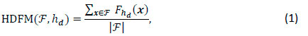
where h_d denotes the Hamming distance at which the neighbourhood N(x) of randomly generated solution χ is considered, and F_hd(x) denotes the proportion of feasible neighbourhood solutions in N(x). A scalar value in the range [0,1] is returned, where larger values indicate larger proportions of surrounding neighbourhood feasibility.

3.2. The pocket size measure

The PSM evaluates the local extent of the feasible region (and infeasible region) by executing a feasible state walk through the fitness landscape. A feasible state walk is an iterative process during which a neighbouring solution x' e N(x) is selected at random if the entire neighbourhood N(x) has the same feasibility state as the current solution χ (and thus the initial solution). Once a neighbouring solution of the opposite feasibility state is encountered, the walk is terminated and the PSM is taken as the length of the walk. The PSM procedure for a feasible state walk is provided in Figure 1. For an infeasible state walk, line 3 should be adapted to the entire neighbourhood being infeasible.

 

 

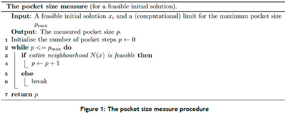
The PSM procedure described in Figure 1 is executed for a set 7 of randomly generated initial solutions (either feasible or infeasible). Thereafter, the measured pocket sizes for all solutions in the set are aggregated to determine the PSM for the set 7. The value returned is a scalar in the range [0, p_max], where p_max acts as a computational limit (selected by the user) for very large pocket sizes. The greater the value returned (i.e., the closer to the aforementioned limit) the greater the extent of the feasible or infeasible region within the fitness landscape.

3.3. The constraint violation severity measure

The CVSM evaluates the degree to which inequality constraints that are imposed are typically violated for the problem instance under consideration - essentially evaluating the tightness of inequality constraints. The CVSM is measured over a set of randomly generated solutions (regardless of feasibility state) with the violation degree of constraint i calculated as

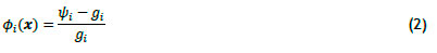
for an inequality of the form ψι(χ) <, > g_i. That is, the degree of constraint violation for each inequality constraint that is imposed is aggregated for the set of randomly generated solutions. The CVSM of an infeasible solution yields a positive scalar value for a less-than-or-equal-to constraint or a negative scalar value for a greater-than-or-equal-to constraint. Therefore, a larger absolute value of the measure indicates a larger degree of constraint violation, perhaps because of a tighter constraint definition.

 

4. THE PAIR SELECTION PROBLEM

The PSP is a binary selection problem in which pairs of items have to be selected from a set P of distinct alternatives in order to maximise a benefit function derived from the pairs of items selected. The selection is required to satisfy a pair inclusion constraint set and a pair exclusion constraint set. Moreover, a collection of subsets of P², called core subsets, is specified, where P² is the set of all (unordered) pairs of distinct elements that can be selected from P. The cost associated with selecting pairs of items from P² is also required to be managed within a specified range for each of these core subsets. The pair selection problem is rather ubiquitous, in the sense that it admits, upon appropriate choices of its parameters and parameter sets, a variety of well-known optimisation problems as special cases, such as the knapsack problem and the quadratic assignment problem.

4.1. Model parameters, variables, and constraints

A benefit b_ij and a cost c_ij- are associated with the selection of item pair {i,j} EP². Moreover, a pair inclusion set T c P² is imposed, specifying that each pair contained in 3 must, in fact, be selected. A pair exclusion set £ c P² is similarly imposed, specifying that no pair contained in £ may be selected. Finally, a collection of core subsets Q₁,.... Q_r is specified, with Q_k cP²\£ for all k = 1,r. The cost of the entire pair selection has to be managed between specified lower and upper bounds for each of these core subsets Q_k.

An upper-triangular binary decision variable matrix X = [x_ij]_{i,j}eP² is employed in the model, where

The constraint sets

and

ensure that the required pairs are included in the solution and that the forbidden pairs are excluded from the solution. Moreover, the constraint set

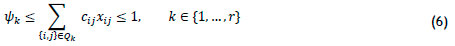
ensures that the costs associated with selecting item pairs from the various core subsets respect the specified budgetary bounds. Note that the above constraints are normalised without loss of generality so that unit upper-cost constraint values are achieved.

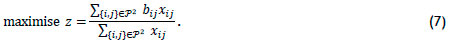
4.2. Model objective

The objective is to maximise the normalised benefit of the pair selection solution - that is, to

 

5. FITNESS LANDSCAPE ANALYTIC OUTPUTS

The significance of the three proposed FLA measures is demonstrated in this section within the context of the PSP. Each measure was evaluated for 40 instances of the PSP, and the results that were obtained are illustrated graphically. This section is partitioned into subsections containing descriptions of the method of generation of the PSP instances and the evaluation of each FLA measure. Feature extraction computations were performed on the high-performance computing cluster of Stellenbosch University (http://www.sun.ac.za/hpc).

5.1. PSP test instance generation

A diverse set of test problem instances was generated for the numerical experiments conducted in this paper. The set comprised 40 problem instances of the PSP, ranging in size and complexity (the latter based on the imposition of constraints). The PSP input parameters were generated according to a mean-centred triangular distribution with empirically tuned limits, as summarised in Table 1.

 

 

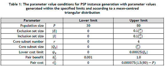
The limits provided in Table 1 were settled upon on the basis of initial empirical testing, with the general aim of pursuing reasonable computation times for the FLA measures that were implemented and the SA metaheuristic configurations that were considered. Moreover, the limits of the constraint sets were tuned to ensure sufficient levels of solution infeasibility (and solution feasibility) in the fitness landscape, such that varying levels of test problem complexity could be achieved.

5.2. The Hamming distance feasibility measure

The HDFM was evaluated at a Hamming distance of 1 for a set 7 of one thousand randomly generated solutions, regardless of feasibility state. The set 7 was partitioned into two subsets, based on the feasibility state of the solutions generated. The HDFM was subsequently calculated for each feasibility subset, resulting in two HDFMs for each test problem instance. To provide additional insight into the extracted HDFMs, the feasibility proportions of the set 7 were recorded, as well as whether any fully infeasible neighbourhoods (for which F_hd (x) = 0) were detected. Infeasible pockets were detected to be surrounding only infeasible solutions. The results are presented graphically in Figure 2, in which the vertical axis was scaled according to the reciprocal of the hyperbolic tangent function (tanh) so as to better elucidate HDFM values closer to the extremal values 0 and 1.

 

 

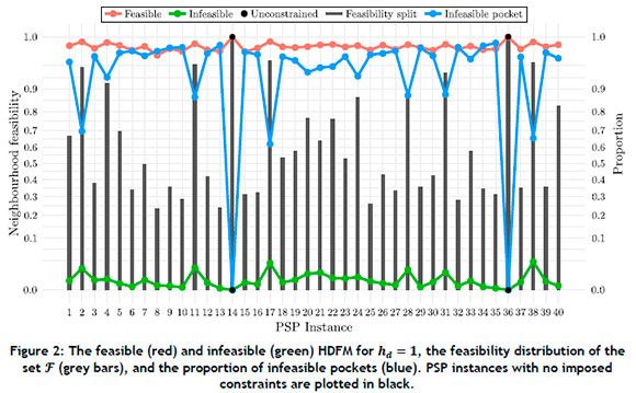
It may be observed in Figure 2 that feasible solutions to the test instances of the PSP exhibited considerably larger proportions of neighbourhood feasibility than did infeasible solutions, with the smallest observed HDFM value for feasible solutions being 0.987 (and achieving an average value of 0.996). The largest observed HDFM value for infeasible solutions, on the other hand, was 0.030 (and achieved an average value of 0.005).

The proportions of feasibility and infeasible pockets provide interesting insight into the nature of the fitness landscapes of the test problems. A trend may be observed among the test problem instances: for instances with larger feasibility splits (i.e., as the feasible subset of 7 increases in size), the HDFM increases for both feasible and infeasible solutions while the proportion of infeasible pockets decreases, suggesting that the feasible region is better connected and more dominant in the fitness landscape for those instances.

The HDFM results also suggest that the PSP test instances exhibited clear boundaries between feasibility regions, as solutions are typically and predominantly surrounded by solutions of the same feasibility state, motivating the consideration of a CHT as part of metaheuristic configuration for scenarios in which infeasible solutions are encountered during the search.

5.3. The pocket size measure

The PSM was evaluated for two sets (one feasible and one infeasible), each containing one thousand randomly generated solutions computed with a computational limit of p_max = 150. The proportions of zero pocket sizes were also recorded during the extraction process. As a result, the extraction process yielded multiple numerical values: the PSMs for the feasible and infeasible solutions, and the zero pocket proportions for the feasible and infeasible sets.

The PSMs and the zero pocket proportions are presented in Figure 3 and Figure 4 respectively for all 40 test problem instances, with the vertical axis in Figure 4 scaled according to the square-root function, so as to visualise smaller zero pocket proportions better.

 

 

 

 

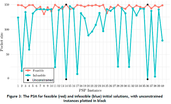
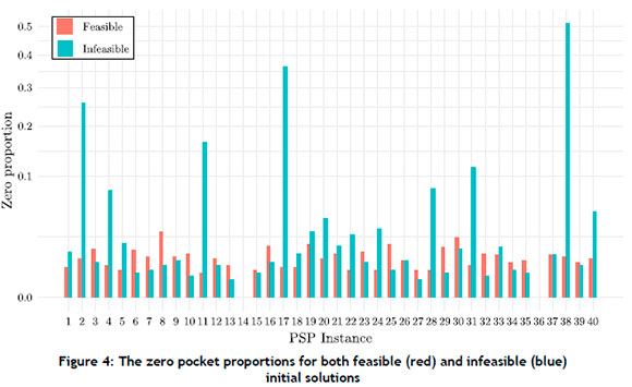
It may be observed in Figure 3 that the feasible regions of the PSP test instances were typically better connected than the infeasible regions, because the feasible PSM was larger than the infeasible PSM in most instances. Even for test problem instances with larger infeasible PSMs (such as for instances 13 and 15), the feasible PSMs remain large, suggesting that feasible regions remain connected even in the presence of extensive infeasible regions. Smaller infeasible PSMs (such as for instances 2, 4, 11, 17, 28, 31, 38 and 40) are likely because of the presence of significantly larger proportions of zero pockets, as illustrated in Figure 4.

The results show that the feasible regions typically exhibited a greater extent in the fitness landscape than the infeasible regions. Interestingly, the PSM was closely linked to the presence of zero pockets, as the PSM values in Figure 2 related to the zero pocket proportions in Figure 3. This shows that pockets are typically very large, with the proportions of zero pockets being a strong factor in measuring smaller PSMs.

5.4. The constraint violation severity measure

The CSVM was evaluated for a set of one thousand randomly generated solutions, regardless of their feasibility status. The violation degree for each infeasible solution in the set was evaluated and aggregated for each inequality constraint that was imposed. As a result, the extraction process yielded multiple numerical values for each constraint (up to a maximum of eight). The greater-than-or-equal-to CVSM values are illustrated in Figure 5, with smaller values (close to zero and negative) indicative of tighter constraints, and the less-than-or-equal-to CSVM values illustrated in Figure 6, with larger positive values indicative of tighter constraints. The vertical axis in Figure 5 was scaled according to the square-root function for visualisation purposes.

 

 

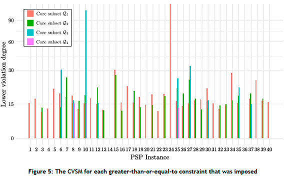
The results referred to above are presented in grouped barplots (because between 0 and 4 core subsets were imposed, and had to be inspected individually) with the CVSM of each inequality constraint shown. As mentioned in Section 3.3, a positive value represents the degree of violation of a less-than-or-equal-to inequality constraint by an infeasible solution, while a negative value represents the degree of violation of a greater-than-or-equal-to inequality constraint by an infeasible solution. The positive violation values in Figure 5, and the negative values in Figure 6, identify constraints as rarely violated, while the positive violation values in Figure 6 identify constraints as easily violated.

 

 

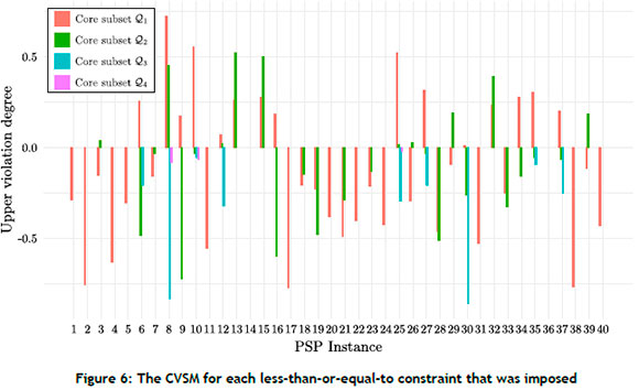
It may be observed in Figure 5 and Figure 6 that greater-than-or-equal-to inequality constraints are typically easier to satisfy than less-than-or-equal-to inequality constraints in the pSp test instances. The figures easily and legibly illustrate the degree of tightness of each - as may be seen for the loose greater-than-or-equal-to constraints in instances 10 and 24, as well as the tight less-than-or-equal-to constraints in instances 8, 10 and 25. Moreover, the results illustrate that not all constraints represent the same degree of tightness, and indicate which constraints are the key regulators of solution infeasibility in the fitness landscape.

 

6. METAHEURISTIC CONFIGURATION SELECTION

The utility of the three newly proposed FLA measures as meta-features for metaheuristic configuration selection is demonstrated in the context of a case study in this section. The case study relates to the classification power of selecting the best-performing CHT when the newly proposed FLA measures are included as meta-features for the construction of a meta-learning model. Two machine-learning classification models are compared (one excluding the novel FLA measures and one including them) and the potential classification performance improvement is evaluated. The classification models are derived from a ranger model, a fast-implementation variant of the well-known random forest model [32]. Jankovic et al. [33] claimed that random forests perform best in the context of algorithmic runtime prediction, thus motivating our implementation choice in this paper.

The remainder of this section is partitioned into subsections devoted to a description of the steps performed during the comparative study and a presentation and discussion of the results. All meta-feature extraction and optimisation performance collection was performed on the high-performance computing cluster of Stellenbosch University (http://www.sun.ac.za/hpc).

6.1. Experimental setup

Numerical experimentation was performed on the 40 PSP test instances described in Section 5.1, partitioning this test set into 30 training instances and 10 validation instances. The meta-features that were considered comprised a variety of general problem descriptors and statistical measures (taken from Table 1) in conjunction with eight FLA measures (five traditional measures, namely autocorrelation [7], correlation length [7], the first and second entropic measures [8], Hamming distance in a level [9], and accumulated escape probability [10], as well as the three novel measures proposed in this paper). The algorithm portfolio included the well-known SA algorithm equipped with a variety of functionality options and hyper-parameter configurations, as summarised in Table 2.

 

 

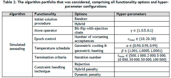
The random initial solution procedure in Table 2 involves generating a random solution, whereas the hybrid procedure involves conducting a limited local search to generate a potentially superior solution over the random procedure. The move operator is a simple bit-flip embedded in a global ejection chain operator [34]. The ejection chain move is implemented stochastically, based on the (reducing) exponential probability:

where t denotes the current iteration number and γ denotes a tunable hyper-parameter controlling the rate of probability decrease; a single bit-flip move is implemented otherwise. The search epochs are delimited by the number of worsening acceptances c_max and the number of worsening rejections, set to d_max = 1.5 · c_max. The search temperature is controlled by geometric cooling with a rate parameter a or geometric reheating, with a rate parameter β at the end of each epoch. The search is terminated upon having completed t_max iterations. Finally, three CHTs are implemented, including rejection according to which infeasible solutions are rejected, a hybrid penalty according to which infeasible solutions are penalised based on the number of constraint violations ν relative to the number of constraints r, and a dynamic penalty according to which infeasible solutions are penalised based on the iteration number t. The corresponding penalty terms are tabulated in Table 3.

 

 

The resulting algorithm portfolio comprised 3 888 distinct variants of the SA algorithm for which optimisation performance measures were collected (in respect of the objective function value (7)).

6.2. Numerical benchmarking results

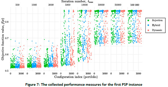
The optimisation performance measures (for the 3 888 algorithmic configuration variants per PSP test instance) were collected and processed to form training and validation databases. An extract of the optimisation performances for the first PSP test instance is presented in Figure 7, where the vertical axis represents the objective function value (i.e., solution quality) and the horizontal axis discretises the algorithm portfolio, based on the different termination criteria. The objective function value can be seen to improve over longer search durations. The points in the figure are grouped according to the CHT that was employed, yielding a wide distribution of optimisation performance for the algorithm portfolio. As observed in this extract, it is not obvious which CHT is most appropriate.

 

 

Once both databases had been generated, they were processed for a classification machine-learning problem. This was achieved by filtering the algorithm portfolio according to the best-performing CHT class for each distinct algorithmic configuration in the problem instance. The result was a condensed portfolio with the best-performing CHT class set as the target variable. An important consideration in a classification problem is the class imbalance of the training database. This imbalance is illustrated graphically in Figure 8 as the CHT proportions of each CHT class.

 

 

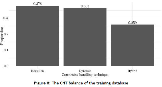
Due to each configuration variant in the database providing valuable information for a particular test problem instance, neither over-sampling nor under-sampling could be performed so as to reduce the risk of overfitting without removing valuable information. Given that no considerable class imbalance was present in the training data, however, the classification models were subsequently trained on the database without any attempt to redress the (small degree of) class imbalance present in the data.

6.3. Classification model training

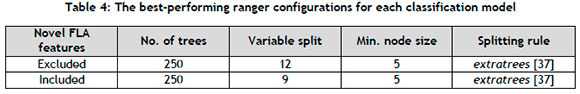
It is well known that feature selection improves random forest prediction performance [35]. Therefore, the 28 most prominent features were selected on the basis of sets of feature importance scores for each classification model (with both models having an equal number of meta-features at their disposal). Interestingly, ten numerical values extracted from the three novel FLA measures were selected. Another advantage of feature selection is that it leads to shorter computation times for hyper-parameter tuning and validation testing.

Thereafter, the best-performing hyper-parameter configuration (based on classification accuracy) was uncovered for each classification model by performing five iterations of leave-one-out cross-validation [36] - where five random instances from the training set were excluded in each fold. This method was implemented over the popular k-fold cross-validation, as the tuned models would only be required to classify a single problem instance at a time. The final hyper-parameter configurations obtained for each classification model are presented in Table 4.

 

 

6.4. Classification results and discussion

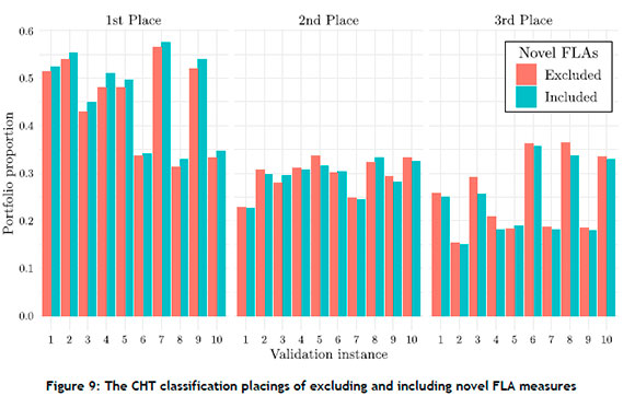
Both tuned classification models were applied to each of the ten validation instances. The resulting classification accuracies and F1 scores are summarised in Table 5. Accuracy refers to the proportion of correctly selected CHTS, while the F1 score is the harmonic mean of the precision and recall metrics. An additional and insightful view of the classification accuracy is illustrated in Figure 9, where the proportions of all placing selections are presented in a grouped barplot. The placing selection refers to whether the predicted CHT is placed first, second, or third out of the possible classes. Therefore, the classification models aim to achieve the most first-place selections, fewer second-place selections, and the least third-place selections.

 

 

 

 

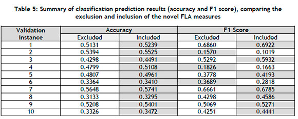
It may be observed in Table 5 and Figure 9 that the inclusion of the novel FLA measures increased the classification power of the ranger classification model. The classification accuracy increased for each validation instance, and the F1 score improved for seven of the ten instances when the novel FLA measures were included as meta-features. This demonstrates the utility of these measures in a meta-learning and algorithm selection context.

Due to the classification accuracies of both models being relatively low, Figure 9 was generated to gain insight into the placings of each model rather than simply the CHT class being correctly or incorrectly identified. This highlights the true utility of classification models in guiding an analyst during metaheuristic configuration selection. It can be seen in Figure 9 that, for every validation instance, the proportion of first-place selections was increased, and that, for nine instances, the third-place selections were reduced, showing that the overall metaheuristic configuration selection abilities were improved by the inclusion of the novel FLA measures.

 

7. CONCLUSION

In this paper we presented three novel fitness landscape measures that were capable of yielding valuable insights into the feasible and infeasible domains of the fitness landscape under consideration. These measures extracted numerical values that may be used to describe various perspectives of both feasible and infeasible solution structures. Numerical experiments were conducted that demonstrated the value of each measure when analysing constrained combinatorial optimisation problems. We also demonstrated in a case study that the inclusion of our novel FLA measures as meta-features improved the classification performance (between 1.37% and 6.44%) of ranger classification models during the task of identifying the best-performing CHTs for the SA algorithm when solving instances of the PSP.

An interesting topic for future experimentation would be to test the utility of the newly proposed FLA measures in the analysis of optimisation problems other than the PSP.

 

REFERENCES

[1] S. Wright, "The roles of mutation, inbreeding, crossbreeding, and selection in evolution," in Proc. 6th International Congress on Genetics, 1932, pp. 356-366.         [ Links ]

[2] S. Wright, "Surfaces of selective value revisited," The American Naturalist, vol. 131, no. 1, pp. 115123, 1988.         [ Links ]

[3] J. P. Watson, "An introduction to fitness landscape analysis and cost models for local search," in Handbook of metaheuristics, M. Gendreau and J. Y. Potvin, Eds. Boston (MA): Springer, 2010, pp. 599-623.         [ Links ]

[4] K. M. Malan and A. P. Engelbrecht, "A survey of techniques for characterising fitness landscapes and some possible ways forward," Information Sciences, vol. 241, pp. 148-163, 2013.         [ Links ]

[5] K. M. Malan, J. F. Oberholzer, and A. P. Engelbrecht, "Characterising constrained continuous optimisation problems," in Proc. Congress on Evolutionary Computation, 2015, pp. 1351-1358.         [ Links ]

[6] P. F. Stadler, "Fitness landscapes," in Biological evolution and statistical physics, M. Lässig and A. Valleriani, Eds. Berlin, Heidelberg: Springer, 2002, pp. 183-204.         [ Links ]

[7] E. Weinberger, "Correlated and uncorrelated fitness landscapes and how to tell the difference," Biological Cybernetics, vol. 63, no. 5, pp. 325-336, 1990.         [ Links ]

[8] V. K. Vassilev, "An information measure of landscapes," in Proc. 7th International Conference on Genetic Algorithms, 1997, pp. 49-56.         [ Links ]

[9] M. Belaidouni and J. K. Hao, "Landscapes and the maximal constraint satisfaction problem," in Artificial evolution, C. Fonlupt, J. K. Hao, E. Lutton, M. Schoenauer, and E. Ronald, Eds. Berlin: Springer, 2000, pp. 244-255.         [ Links ]

[10] G. Lu, J. Li, and X. Yao, "Fitness-probability cloud and a measure of problem hardness for evolutionary algorithms," in Proc. Evolutionary Computation in Combinatorial Optimization, 2011, pp. 108-117.         [ Links ]

[11] K. M. Malan, "A survey of advances in landscape analysis for optimisation," Algorithms, vol. 14, no. 2, Manuscript 40, 2021.         [ Links ]

[12] M. Dorigo, "Optimisation, learning and natural algorithms," PhD thesis, Politecnico di Milano, Milan, 1992.         [ Links ]

[13] S. Kirkpatrick, C. D. Gelatt, and M. P. Vecchi, "Optimization by simulated annealing," Science, vol. 220, no. 4598, pp. 671-680, 1983.         [ Links ]

[14] S. K. Joshi and J. C. Bansal, "Parameter tuning for meta-heuristics," Knowledge-Based Systems, vol. 189, Manuscript 105094, 2020.         [ Links ]

[15] A. Petrow, "Constraint-handling techniques for highly constrained optimization," Master's thesis, Otto-von-Guericke University, Magdeburg, Germany, 2019.         [ Links ]

[16] J. R. Rice, "The algorithm selection problem," in Advances in computers, vol. 15, M. Rubinoff and M. C. Yovits, Eds. New York (NY): Academic Press, 1976, pp. 65-118.         [ Links ]

[17] L. Xu, F. Hutter, H. H. Hoos, and K. Leyton-Brown, "SATzilla: Portfolio-based algorithm selection for SAT," Journal of Artificial Intelligence Research, vol. 32, pp. 565-606, 2008.         [ Links ]

[18] M. Lindauer, H. H. Hoos, F. Hutter, and T. Schaub, "AutoFolio: An automatically configured algorithm selector," Journal of Artificial Intelligence Research, vol. 53, pp. 745-778, 2015.         [ Links ]

[19] H. H. Hoos, "Automated algorithm configuration and parameter tuning," in Autonomous search, Y. Hamadi, E. Monfroy, and F. Saubion, Eds. Berlin: Springer, 2012, pp. 37-71.         [ Links ]

[20] K. A. Smith-Miles, "Cross-disciplinary perspectives on meta-learning for algorithm selection," ACM Computing Survey, vol. 41, no. 1, Manuscript 6, 2009.         [ Links ]

[21] L. Kotthoff, "Algorithm selection for combinatorial search problems: A survey," AI Magazine, vol. 35, no. 3, pp. 48-60, 2014.         [ Links ]

[22] P. Kerschke, H. H. Hoos, F. Neumann, and H. Trautmann, "Automated algorithm selection: Survey and perspectives," Evolutionary Computation, vol. 27, no. 1, pp. 3-45, 2019.         [ Links ]

[23] E. Nudelman, K. Leyton-Brown, H. H. Hoos, A. Devkar, and Y. Shoham, "Understanding random SAT: Beyond the clauses-to-variables ratio," in Proc. 10th International Conference on the Principles and Practice of Constraint Programming, 2004, pp. 438-452.         [ Links ]

[24] A. E. Howe, E. Dahlman, C. Hansen, M. Scheetz, and A. von Mayrhauser, "Exploiting competitive planner performance," in Proc. 5th European Conference on Planning, 1999, pp. 62-72.         [ Links ]

[25] D. I. Seo and B. R. Moon, "An information-theoretic analysis on the interactions of variables in combinatorial optimization problems," Evolutionary Computation, vol. 15, no. 2, pp. 169-198, 2007.         [ Links ]

[26] K. A. Smith-Miles and J. van Hemert, "Discovering the suitability of optimisation algorithms by learning from evolved instances," Annals of Mathematics and Artificial Intelligence, vol. 61, no. 2, pp. 87-104, 2011.         [ Links ]

[27] C. Fawcett, M. Vallati, F. Hutter, J. Hoffmann, H. H. Hoos, and K. Leyton-Brown, "Improved features for runtime prediction of domain-independent planners," in Proc. 24th International Conference on Automated Planning and Scheduling, 2014, pp. 355-359.         [ Links ]

[28] K. A. Smith-Miles, "Towards insightful algorithm selection for optimisation using meta-learning concepts," in Proc. IEEE International Joint Conference on Neural Networks, 2008, pp. 4118-4124.         [ Links ]

[29] E. Pitzer, A. Beham, and M. Affenzeller, "Automatic algorithm selection for the quadratic assignment problem using fitness landscape analysis," in Evolutionary computation in combinatorial optimization, M. Middendorf and C. Blum, Eds. Berlin: Lecture Notes in Computer Science, Volume 7832, Springer, 2013, pp. 109-120.         [ Links ]

[30] A. Dantas and A. Pozo, "On the use of fitness landscape features in meta-learning based algorithm selection for the quadratic assignment problem," Theoretical Computer Science, vol. 805, pp. 6275, 2020.         [ Links ]

[31] A. Liefooghe, F. Daolio, S. Verel, B. Derbel, H. Aguirre, and K. Tanaka, "Landscape-aware performance prediction for evolutionary multiobjective optimization," IEEE Transactions on Evolutionary Computation, vol. 24, no. 6, pp. 1063-1077, 2020.         [ Links ]

[32] L. Breiman, "Random forests," Machine Learning, vol. 45, pp. 5-32, 2001.         [ Links ]

[33] A. Jankovic, G. Popovski, T. Eftimov, and C. Doerr, "The impact of hyper-parameter tuning for landscape-aware performance regression and algorithm selection," in Proc. Genetic and Evolutionary Computation Conference, 2021, pp. 687-696.         [ Links ]

[34] F. Glover, "Ejection chains, reference structures and alternating path methods for traveling salesman problems," Discrete Applied Mathematics, vol. 65, no. 1, pp. 223-253, 1996.         [ Links ]

[35] A. Jankovic and C. Doerr, "Landscape-aware fixed-budget performance regression and algorithm selection for modular CMA-ES variants," in Proc. Genetic and Evolutionary Computation Conference, 2020, pp. 841-849.         [ Links ]

[36] T. T. Wong, "Performance evaluation of classification algorithms by k-fold and leave-one-out cross validation," Pattern Recognition, vol. 48, no. 9, pp. 2839-2846, 2015.         [ Links ]

[37] P. Geurts, D. Ernst, and L. Wehenkel, "Extremely randomized trees," Machine Learning, vol. 63, no. 1, pp. 3-42, 2006        [ Links ]

 

 

* Corresponding author: nathan.vdw19@gmail.com
ORCID® identifiers
N.J. van der Westhuyzen: https://orcid.org/0009-0007-5298-109X
J.H. van Vuuren: https://orcid.org/0000-0003-4757-5832