CASE STUDIES

 

Inventory management with stochastic demand: case study of a medical equipment company

 

 

R. Ternero^{I, II}; J.P. Sepúlveda-Rojas^I; M. Alfaro^I; G. Fuertes^{I, III, *}; M. Vargas^I

^IIndustrial Engineering Department, University of Santiago, Chile
^IIEscuela de Construcción, Universidad de las Américas, Chile
^IIIFacultad de Ingeniería, Ciencia y Tecnología, Universidad Bernardo O'Higgins, Chile

 

 

---

ABSTRACT

This research proposes an inventory management system based on a periodic review model for a medical equipment company. The work aims to reduce inventory volume and out-of-stock and to improve service levels. The proposed methodology is a combined ABC/XYZ classification using the patterns and magnitude of demand under the constraints of spare parts cost. For the ABC/XYZ classification, we propose a model to forecast demand; and we evaluate eight forecasting methods to adjust the classification characteristics. The results obtained allow the reduction of arrears, an increased service level, and a decrease in average inventory.

---

OPSOMMING

Hierdie navorsing stel 'n voorraadbestuurstelsel voor wat gebaseer is op 'n periodieke hersieningsmodel vir 'n mediese toerustingmaatskappy. Die werk het ten doel om voorraadvolume en geen voorraad situasies te verminder en diensvlakke te verbeter. Die voorgestelde metodologie is 'n gekombineerde ABC/XYZ-klassifikasie wat die patrone en omvang van die vraag gebruik onder die beperkings van onderdelekoste. Vir die ABC/XYZ-klassifikasie stel ons 'n model voor om vraag te voorspel; en ons evalueer agt voorspellingsmetodes om die klassifikasie-eienskappe aan te pas. Die resultate wat verkry is, laat die vermindering van agterstallige voorraad, 'n verhoogde diensvlak, en 'n afname in gemiddelde voorraad toe.

---

 

 

1. INTRODUCTION

Inventory management models seek a balance in the level of stock according to the reality faced by companies and their demands to reduce the different costs that might be incurred [1]. The Pareto principle, known as the 80-20 rule, serves as the basis for ABC analysis and XYZ analysis. ABC inventory classification is a technique for segmenting entities (products, customers, suppliers, etc.). Douissa and Jabeur [2] applied this principle in a warehouse to classify stock-keeping units (SKUs) according to their importance, and arranged them into three categories - category A (very important SKU), category B (moderately important SKU), and category C (relatively unimportant SKU) - which were classified on the basis of the demand volume or demand value (valued sale). According to Pérez Vergara et al. [3], one of the most frequently used classifications is 20%, 30%, and 50% for products A, B, and C respectively.

ABC/XYZ analysis is used to generate production, inventory control, and supply strategies that are useful for optimising merchandise stock. The XYZ classification corresponds to a combination of the result of two ABC classifications. SKUs that were classified as important in both ABC classifications, with regular and constant demands, would have an X classification. SKUs classified as less important, classified as Y, would have some predictable fluctuations (seasonality, trend, or economic factors); therefore, future demand forecasts would be less reliable for these items. Finally, those SKUs classified as unimportant, with irregular or even stochastic demands, would be classified as Z [4]. Different authors have used the ABC/XYZ analysis in the pharmaceutical industry [5], manufacturing [6], the construction industry [7], and trading companies [8]. In this study, we used the aBc/XYZ analysis to understand better the groups made up of SKUs, taking into account the category and the demand pattern.

Numerous time series prediction models have been proposed in recent decades [9]-[12]. Two main types of prediction methods (linear statistical models and non-linear time series models) are well-studied and investigated in the literature [13]. The biggest problem with forecasting demand is its stochastic character, which limits long-term forecasting capabilities. Accurate demand forecasting is a critical factor in determining the quality of decision-making. A poor forecast causes unnecessary costs to the supply chain; therefore, appropriate strategies are needed to keep demand volatility in check.

Different research teams have proposed techniques to control demand. Increased inventory levels impose costs on the company and increase supply capacity. These approaches could address problems associated with demand volatility; however, they could also reduce business profitability, depending on the circumstances.

Demand forecasting is the first requirement for controlling demand volatility. There is no single universal forecasting model for all specific problems. However, some models perform better under certain conditions. For example, Abolghasemi et al. [14] used ARIMA (autoregressive integrated moving average) , ARIMAX (an extension of the ARIMA model), eTs (error-trend-seasonality), ETSX (an extension of ETS), exponential smoothing with covariate, dynamic linear regression (DLR) and proposed a hybrid model to forecast highly volatile demands. Huang et al. [15] proposed two methods - ADL (autoregressive distributed lag)-intra-EWC (estimation window combining), and ADL-intra-IC (intercept correction) - to forecast the sales of retail products while taking structural change problems into account. Continuing with the retail product sales forecast at the SKU level, Ali et al. [16] proposed the regression tree method with a range of variables constructed from sales, price, and product promotion. Hyndman and Athanasopoulos [17] proposed the use of two popular extrapolative models, ARIMA and exponential smoothing. These methods base their forecasts on extrapolations of past patterns; however, pattern changes can seriously compromise their effectiveness. Authors such as Bata et al. [18] developed an artificial neural network (ANN) model to forecast water demand 24 hours and one week in advance. The results showed that a non-linear ANN model can improve water demand prediction by 18% and 25% respectively. Spiliotis et al. [19] propose using machine learning (ML) methods for the daily forecasting of SKU demand as an alternative to statistical methods. The results indicated that some ML methods provided better prognoses, in respect of both precision and bias. Alfaro et al. [20] proposed the use of two forecasting models (ANN and support vector machine) for the study of three-time series. The forecasting models built with ANN and support vector machine could make good quality forecasts.

This study is divided into five sections. Section 1 introduces the concept of ABC/XYZ classification to evaluate the logistics cost of goods storage - in particular, the demand forecasting models for the correct management of inventories. Section 2 describes the methodology proposed by Cavalieri et al. [21] developed from the ABC classification and the classification proposed by Ghobbar and Friend [22] considering the volume of demand, the cost of spare parts, and demand patterns. Section 3 presents a demand forecasting method adjusted to the characteristics of the proposed classification. Section 4 proposes an inventory management system based on periodic review. Finally, section 5 presents the conclusions of the study.

 

2. METHODOLOGY

2.1. ABC classification

The first classification for spare parts was an ABC classification scheme to determine the relevance of parts in relation to their annual sales volume (cost of SKU x annual sales) [23]. The analysed demand corresponded to the period October 2017 to September 2018, for 2 031 SKUs. The results obtained for the ABC classification are summarised in Table 1.

 

 

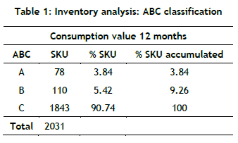
Table 1 shows that the number of products classified as 'A' and 'B' were less than 10% of the total SKUs, even though their valued weight was 95%. As a result, of 2 031 SKUs, only 78 were classified as important category 'A' parts - that is, 3.84% of the parts used in the technical service corresponded to 80% of the total recovery. In category 'B' there were 110 SKUs, corresponding to 5.42% of the total parts; and finally, most of the spare parts were categorised as 'C', with 1 843 SKUs, equivalent to 90.74% of the total number of parts.

2.2. Classification by demand patterns

The second classification considered the demand patterns for each SKU. The spare parts had months with a demand equal to 0. These characteristics forced us to introduce the demand coefficients of quadratic variation (CV²) and the interval between the average demands (ADI). Thanks to these criteria, a classification could be made into four categories:

1. Soft demand: demand is regular, with few periods of no demand, with a low CV² coefficient and a low ADI.

2. Intermittent demand: it is a bit more random, with little variation in the demand for quantity and a greater variation in the intervals between two demands, with a low CV² coefficient and a high ADI.

3. Erratic demand: it is regular over time, with a high variation in demand. It has a low interval between ADI and a high CV² coefficient of demand.

4. High demand: the variability of the quantity demanded and the intervals are high; the CV² coefficient is high, as is the ADI.

The cut-off points for the parameters used in this classification (CV² and ADI) were established by [22] and are shown in Figure 1. In addition, Figure 2 shows examples of demand patterns for different SKUs used in technical service.

 

 

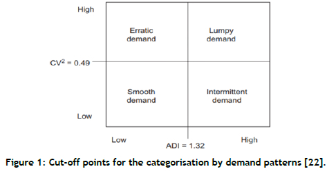
Table 2 summarises the data obtained for classifying the patterns of demand. For the preparation of this classification, we used the same database as for the ABC classification.

 

 

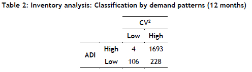
According to Table 2, 106 SKUs - equivalent to 5.22% of the total number of spare parts - were classified as soft demand; 11.23% of the SKUs (228 spare parts) were classified as intermittent demand; four of the 2 031 spare parts used in technical service were classified as erratic demand; and 83.36%, - that is, 1 693 SKUs - were classified as lumpy demand.

2.3. Combined classification

The final classification consisted of a combination of the results obtained previously. For this, we created a table consolidating both classifications, forming a matrix that established different inventory policies for each category, similar to the ABC/XYZ classification proposed by [24]. This combined classification would make it possible to transform the classification of demand type and complexity (XYZ) into classification by demand patterns. The result of the combined classification is shown in Table 3.

 

 

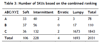
Table 3 shows the importance of the different spare parts used in the job. For example, only 33 of the spare parts fell into the 'A' rating with a soft demand pattern, while 1 673 SKUs fell into the 'C' rating with a lumpy demand pattern, equivalent to 82.37% of the total; this reduced the main analysis to 20% of the total SKUs.

 

3. DEMAND AND FORECAST FOR SPARE PARTS

3.1. Forecasting methods

This section applied the third phase of the framework of Cavalieri et al. [21], making a demand forecast that was adjusted to the spare parts' characteristics (low consumption level, periods of zero demand, and demand variability). The methodology of this study, given the unavailability of data related to forecasts based on the reliability or safety of the spare parts, used forecasts based on time series. Table 4 summarises the forecasting methods used in the time series analysis. In each R software code (third column of table 4) , the variable 'y' represents the time series, and the variable 'h' represents the number of predicted periods, with n = 9 for training and n = 1 for the final forecast.

This study worked with demand forecasting techniques based on time series, owing to the availability of information on the consumption of these items. Once the above was established, the spare parts forecast was made, giving greater importance to the most relevant parts according to the previously performed classification (for example, parts classified as A with a soft demand pattern). Therefore, a different number of methods were applied to each group (Table 5).

A-classified SKUs with a soft demand pattern were the most important combination for the value of parts and their stable demand pattern. Therefore, we applied a greater number of forecasting methods in search of the lowest percentage error.

A-classified SKUs with intermittent and erratic demand patterns had a demand that was difficult to predict; the research used fewer methods. To solve the previous problem, the CROSTON method improved the forecast by smoothing demand [25].

B-classified SKUs had less impact on valuation than A-classified SKUs because fewer forecasting methods were used. SKUs classified as C had little impact on demand volume; therefore, few forecasting methods were used. Finally, for SKUs with a lumpy demand pattern, the CROSTON and naive methods were used for their forecast, owing to the great dispersion and fluctuation of their data.

3.2. Choice of forecast

We used the R software to programme the demand prediction methods. Monthly spare parts demand data was collected for the technical service area between January 2015 and September 2018 - a total period of 45 months, with the first 36 months of data being for the training set and the remaining nine months of data for the test set. To find the best prognosis for each classified group, we programmed each method in the R software.

Once the demand forecasts for each of the spare parts had been found, the most accurate forecasts were chosen. For this, we established the performance and error measures. In general, the mean absolute percentage error (MAPE) is recommended as a measurement method to define which prognosis would be used [26]. However, we used seasonal mean absolute scaled error (MASE) as the performance measure for this work. MAPE could not be used, as it cannot calculate time series with null elements. In our case study, because of intermittent demand, zero demands on spare parts were common. Besides, authors such as Hyndman and Koehler [26] have recommended using MASE as the best available precision measure. Table 6 shows the forecasts with the lowest error for each piece in each classification.

Table 6 shows that the most accurate method for A-classified SKUs with a soft demand pattern was ARIMA, with 42% of the total of 33 pieces in that rating. For A-classified parts with an intermittent and erratic demand pattern, the most widely used methods were ARIMA and SES, with 40% of the total 42 spare parts.

For the pieces classified as B, the most frequently used method was SES, with 57% of the pieces with a soft demand pattern and 60% with an intermittent and erratic demand pattern. For the other specified subsets, the most widely used method was Naive, mainly owing to the low amount of demand in parts classified as C and the dispersion of the data with a lumpy demand pattern.

 

4. INVENTORY MANAGEMENT POLICY

In this section, a new inventory policy is proposed for all SKUs, focusing on the method's performance on spare parts classified as A with a soft demand pattern.

An action policy was used that was based on the periodic review model (order up to level S), which considered the average demand during the delivery period and the review period with the necessary safety stock for that period.

4.1. Development of the fixed-period inventory model

Once we had established the parameters to develop a periodic review policy, taking into account Shah's [27] proposal, this study established the objective inventory (S). This proposal was composed of the forecast demand (D) during the time interval between reviews (R) and the delivery time (L) plus the safety inventory (SS) (equation 1).

where the safety inventory is composed of the safety factor as a function of the desired service level Ζ and the standard deviation of demand (σ_D) during R and L (equation 2).

Equation 2 assumes a fixed delivery time without deviation; it only considers a possible variation in demand. If there is uncertainty in the waiting time, as in our case it is necessary to modify the standard deviation formulation to take account of this new uncertainty and increase the level of the safety inventory (equation 3).

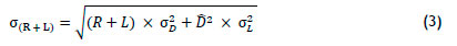
Finally, the target inventory is expressed according to equation 4.

In addition, given the previous calculation of the safety stock, it was possible to approximate the proportion of the demand that was satisfied with the available inventory - that is, the filling rate of each spare part. The expected shortage per replenishment cycle (ESC) was the average number of demand units that were not met by the stored inventory per replenishment cycle. Given a batch size Q, which was the average demand in a replenishment cycle [28], equation 5 expresses the fill rate (fr).

for which the expected shortage in the replenishment cycle is given by equation 6.

where F_s is the cumulative standard normal distribution function and f_s is the standard normal density function.

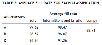
Considering equations 1-6, the average filling rate could be generated for each subset (Table 7).

 

 

4.2. Application of the periodic review model in the case study

Table 8 shows an example of a common service repair. This repair consists of a combination of six spare parts, and the fill rate represents the average fraction of orders that are fulfilled with the available inventory.

 

 

According to Table 8, this repair's fill rate would be 87.98% - a value lower than the individual fill rate of the SKU components; SKU availability enables a response to the repair request.

To compare this example with the real situation, we performed a simulation of the proposed inventory management policy, including the performance indicators of (1) average inventory, (2) business volume, (3) arrears, (4) inventory days, and (5) costs. Table 9 shows the total inventory cost (configuration costs and stock holding) for parts A with a soft demand pattern. The data used corresponded to the period October 2017 to September 2018. We compared the actual policy with the proposed policy.

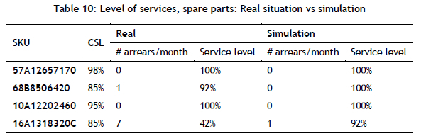
Table 9 shows a decrease in the total cost of the simulated parts by reducing the configuration cost and the stock holding. Based on the new inventory policy, the parts cycle service level (CSL) was maintained or improved compared with the real situation (Table 10).

According to Table 10, the simulated service level for the four exemplified spare parts was maintained or improved compared to the current service level.

Table 11 shows the turnover ratio, inventory days, and the difference between the current situation and the simulation of a sample of spare parts.

Table 11 shows that the four parties' turnover ratio increased from 3.19 to 7.86 with the application of the new inventory policy. The average permanence of spare parts decreased by 0.04. For the SKU 16A1318320C, a value of 0 could occur (some value was missing to calculate the variable based on the formula, or there was no real value in that classification); therefore, no values are presented in the real column.

When performing this analysis on a larger sample (A parts with a soft demand), the difference between the current situation and the simulated turnover ratio and inventory days varied, being positive for some spare parts and negative for others. This was mainly because the proposed new inventory policy decreased backlogs for all spare parts classified as A with soft demand.

Table 12 and Table 13 show the differences between the spare parts classified as A with soft demand (with and without delays) for the real situation and the simulated one.

 

 

 

 

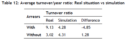
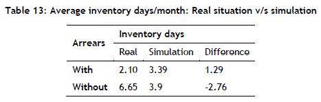
According to Table 12 and Table 13, the average turnover decreased for the spare parts with arrears in the real situation. Also, their average days of inventory increased because the amount of inventory of these parts increased to satisfy demand and eliminate arrears.

This study did not consider the cost of the out-of-stock. Since spare parts were used, the effect of not having them available was to increase the delivery time of the repaired product; and this cost was difficult to quantify in both the current and the proposed situation. Moreover, since medical equipment was used, the cost of out-of-stock could be much higher than the opportunity cost of timely payment, since the health of the patient using this equipment was involved.

The opposite occurred with those spare parts that did not present delays in the real situation. The average rotation ratio increased and their average permanence decreased, thus reducing the inventory of these parts and maintaining their level of service.

Table 14 shows the average monthly inventory of spare parts A with soft demand (real situation vs simulation).

 

 

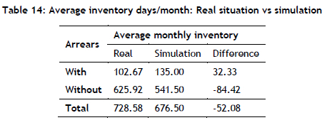
Table 14 shows an increase in the average monthly inventory that, in the real situation, had arrears, to be able to reject it. On the other hand, it decreased for those parts that did not have arrears.

 

5. CONCLUSION

This research has proposed an inventory system using a new periodic review model. Initially, the ABC classification determines the relevance of the pieces in respect of their annual sales volume. Subsequently, we performed classification by demand patterns, depending on variables CV² and ADI (soft, intermittent, erratic, and bulky). To identify the level of importance of the different spare parts, we carried out a combined ABC/XYZ classification; the findings indicated that the 'A' rating with a soft demand pattern and the 'C' rating with a bulky demand pattern performed the best. Validation of the inventory policy was carried out by simulating the model over a 12-month period for our case study. In the simulation for spare parts (real situation: out-of-stock), the average rotation decreased from 9.13 to 4.28 rotations per year and the permanence increased from 2.10 to 3.39, owing to a safety inventory being established to avoid shortages. Regarding spare parts (real situation: with stock) the average rotation increased from 3.02 to 4.31 annual rotations and the permanence decreased from 6.65 to 3.90, owing to the elimination of part of the excess stock. As a result, the simulations allowed reduced arrears, an increased service level, and a decrease in average inventory.

For the demand prediction, a model that used eight statistical methods was proposed (SES, HOLT, HW, MA, ARIMA, CROST, MEAN, and NAIVE). The selection of the forecast statistical method depended on the demand pattern. To calculate the performance and error measures, the MASE method was used, which considers time series with null elements. The period of the data used corresponded to 45 months.

Following the stochastic demand behaviour and the variability in delivery times, this work proposes an inventory management system based on a periodic review model. The proposed inventory policy defines the number of spare parts needed for the safety stock and the order up to level (S), guaranteeing a decrease in backlogs.

Regarding the level of service, CSL was chosen to take the proposed product classification into account. A higher level of service was defined for those parts with a smooth demand pattern and an A rating.

Regarding the average monthly inventory of spare parts, there is a decrease in the total number of parts inventoried monthly, generating greater storage space availability and lower stock holding costs. This new periodic review method reduces the total cost (configuration costs and stock holding), reduces backlogs, increases the service level, and reduces the average inventory compared with traditional inventory management models.

Finally, these recommendations were effectively implemented in a company that repairs medical equipment in Santiago, Chile. Unfortunately, because of time constraints and the ongoing Covid-19 pandemic, it was not possible to verify the effects of the application of these policies. On the other hand, this study was conducted before the pandemic, so the effects of Covid-19 on this proposal study could not be determined with certainty; the same applies to the war in Ukraine. However, in the case of Covid-19, the demand for medical equipment might have increased, which would have led to a drop in demand variability, causing more products to fall into category A with soft demand, thus amplifying that result. In the case of the war in Ukraine, we believe that a disruption in the supply of parts or spare parts would have affected lead times, increased delays, and affected the company's service level.

 

CONFLICTS OF INTEREST

The authors declare that there is no conflict of interest in the publication of this paper.

 

ACKNOWLEDGEMENT

The authors wish to thank DICYT University of Santiago de Chile, Grant 062117SR, for support for this research. This research has been supported by DICYT (Scientific and Technological Research Bureau) of the University of Santiago de Chile (USACH) and the Department of Industrial Engineering.

This research was supported in part by the National Fund for Scientific and Technological Development (FONDECYT, Chile), grant no. 11200993 (MV).

 

REFERENCES

[1] Fuertes, G., Alfaro, M., Soto, I., Carrasco, R., Iturralde, D., & Lagos, C. 2018. Optimization model for location of RFID antennas in a supply chain. In IEEE International Conference on Computers Communications and Control, pp. 203-209.         [ Links ]

[2] Douissa, M. R., & Jabeur, K. 2020. A non-compensatory classification approach for multi-criteria ABC analysis. Soft Computing, 24(13), pp. 9525-9556.         [ Links ]

[3] Pérez Vergara, I. G., Arias Sánchez, J. A., Poveda-Bautista, R., & Diego-Mas, J. A. 2020. Improving distributed decision making in inventory management: A combined ABC-AHP approach supported by teamwork. Complexity (Article ID 6758108), pp. 1-13.         [ Links ]

[4] Aktunc, E. A., Basaran, M., Ari, G., Irican, M., & Gungor, S. 2019. Inventory control through ABC/XYZ analysis. In Industrial engineering in the big data era, F. Calisir, E. Cevikcan, and H. Camgoz Akdag, Eds., Springer, pp. 175-187.         [ Links ]

[5] Bialas, C., Revanoglou, A., & Manthou, V. 2020. Improving hospital pharmacy inventory management using data segmentation. American Journal of Health-System Pharmacy, 77(5), pp. 371-377.         [ Links ]

[6] Zenkova, Z., & Kabanova, T. 2018. The ABC-XYZ analysis modified for data with outliers. In IEEE International Conference on Logistics Operations Management, pp. 1-6.         [ Links ]

[7] Konikov, A., & Konikov, G. 2016. Methodology of construction site marketing analysis. In Procedia Engineering, vol. 165, pp. 1052-1056.         [ Links ]

[8] Stoll, J., Kopf, R., Schneider, J., & Lanza, G. 2015. Criticality analysis of spare parts management: A multi-criteria classification regarding a cross-plant central warehouse strategy. Production Engineering, 9(2), pp. 225-235.         [ Links ]

[9] Carrasco, R., Vargas, M., Soto, I., Fuertes, G., & Alfaro, M. 2015. Copper metal price using chaotic time series forecasting. IEEE Latin America Transactions, 13(6), pp. 1961-1965.         [ Links ]

[10] De Gooijer, J. G., & Hyndman, R. J. 2005. 25 years of IIF time series forecasting: A selective review. Tinbergen Institute Discussion Paper No TI2005-068/4, pp. 5-68.         [ Links ]

[11] Lagos, C., Carrasco, R., Soto, I., Fuertes, G., Alfaro, M., & Vargas, M. 2018. Predictive analysis of energy consumption in mining for making decisions. In IEEE International Conference on Computers Communications and Control, pp. 270-275.         [ Links ]

[12] Carrasco, R., Vargas, M., Soto, I., Fuentealba, D., Banguera, L., & Fuertes, G. 2018. Chaotic time series for copper's price forecast. In Digitalisation, innovation, and transformation, Liu, K., Nakata, K., Li, W., Baranauskas, C. (eds), vol.527, Springer, pp. 278-288.         [ Links ]

[13] Ben Taieb, S., Bontempi, G., Atiya, A. F., & Sorjamaa, A. 2012. A review and comparison of strategies for multi-step ahead time series forecasting based on the NN5 forecasting competition. Expert Systems with Applications, 39(8), pp. 7067-7083.         [ Links ]

[14] Abolghasemi, M., Beh, E., Tarr, G., & Gerlach, R. 2020. Demand forecasting in supply chain: The impact of demand volatility in the presence of promotion. Computers and Industrial Engineering, 142, 106380.         [ Links ]

[15] Huang, T., Fildes, R., & Soopramanien, D. 2019. Forecasting retailer product sales in the presence of structural change. European Journal of Operational Research, 279(2), pp. 459-470.         [ Links ]

[16] Ali, Ö. G., Sayin, S., Van Woensel, T., & Fransoo, J. 2009. SKU demand forecasting in the presence of promotions. Expert Systems with Applications, 36(10), pp. 12340-12348.         [ Links ]

[17] Hyndman, R. J., & Athanasopoulos, G. 2018. Forecasting: Principles and practice (2nd ed.). Melbourne, Australia: OTexts.         [ Links ]

[18] Bata, M. H., Carriveau, R., & Ting, D. S.-K. 2020. Short-term water demand forecasting using nonlinear autoregressive artificial neural networks. Journal of Water Resources Planning and Management, 146(3), pp. 1-9.         [ Links ]

[19] Spiliotis, E., Makridakis, S., Semenoglou, A. A., & Assimakopoulos, V. 2020. Comparison of statistical and machine learning methods for daily SKU demand forecasting. Operational Research, vol. 22, no. 3, pp. 3037-3061.         [ Links ]

[20] Alfaro, M., Fuertes, G., Vargas, M., Sepúlveda, J., & Veloso-Poblete, M. 2018. Forecast of chaotic series in a horizon superior to the inverse of the maximum Lyapunov exponent. Complexity (Article ID 1452683), pp. 1-9.         [ Links ]

[21] Cavalieri, S., Garetti, M., Macchi, M., & Pinto, R. 2008. A decision-making framework for managing maintenance spare parts. Production Planning & Control, 19(4), pp. 379-396.         [ Links ]

[22] Ghobbar, A. A., & Friend, C. H. 2002. Sources of intermittent demand for aircraft spare parts within airline operations. Journal of Air Transport Management, 8(4), pp. 221-231.         [ Links ]

[23] Dhillon, B. S. 2002. Engineering maintenance: A modern approach. New York, NY: Taylor & Francis Group.         [ Links ]

[24] Errasti, A., Chackelson, C., & Poler, R. 2010. An expert system for inventory replenishment optimization. In IFIPAdvances in Information and Communication Technology, Á. Ortiz, R. D. Franco, and P. G. Gasquet, Eds., Berlin: Springer, 2010,pp. 129-136.         [ Links ]

[25] Croston, J. D. 1972. Forecasting and stock control for intermittent demands. Operational Research Quarterly, 23(3), pp. 289-303.         [ Links ]

[26] Hyndman, R. J., & Koehler, A. B. 2006. Another look at measures of forecast accuracy. International Journal of Forecasting, 22(4), pp. 679-688.         [ Links ]

[27] Shah, J. 2009. Supply chain management: Text and case, 1st ed., New Delhi,India: Pearson Education.         [ Links ]

[28] Chopra, S., & Meindl, P. 2013. Supply chain management: Strategy, planning, and operation. Boston MA: Pearson Education.         [ Links ]

 

 

Submitted by authors 28 Oct 2021
Accepted for publication 18 Nov 2022
Available online 26 May 2023

 

 

* Corresponding author: guillermo.fuertes@usach.cl
ORCID® identifiers
R. Ternero: https://orcid.org/0000-0002-6075-6657
J.P. Sepúlveda-Rojas: https://orcid.org/0000-0002-6725-7295
M. Alfaro: https://orcid.org/0000-0002-1633-8853
G. Fuertes: https://orcid.org/0000-0003-3044-5919
M. Vargas: https://orcid.org/0000-0003-4161-6621