GENERAL ARTICLES

 

Three-step sequential compound real options method for electricity capacity expansion

 

 

M. Bashe^*; M. Shuma-Iwisi; M.A. van Wyk

School of Electrical and Information Engineering, University of the Witwatersrand, South Africa

 

 

---

ABSTRACT

A three-step sequential compound real options (SCRO) method is developed and applied to the South African technology for fluidised bed combustion with carbon capture and storage (FBCwCCS). The objective of this paper is to address the plan's implementation when electricity demand is uncertain. The SCRO results are compared with the net present value (NPV) approach. The data for both the SRCO and the NPV is extracted from the mixed integer two-stage stochastic programming results. Negative NPV results indicate that the investment for the FBCwCCS should be rejected. The SCRO results suggest that decisionmakers can exercise the option to invest if the start-up costs are less than or equal to R130 million, or otherwise defer the FBCwCCS investment projects. The industry lags behind in implementing the real option models; the same is expected with the SCRO models.

---

OPSOMMING

'n Drie-stap sekwensiële saamgestelde reële opsies (SCRO) metode is ontwikkel en toegepas op die Suid-Afrikaanse tegnologie vir vloeibedverbranding met koolstofopvang en -berging (FBCwCCS). Die doel van hierdie artikel is om die plan se implementering aan te spreek wanneer die vraag na elektrisiteit onseker is. Die SCRO resultate word vergelyk met die netto huidige waarde (NHW) benadering. Die data vir beide die SRCO en die NHW word uit die gemengde heelgetal tweestadium stogastiese programmeringsresultate onttrek. Negatiewe NHW-resultate dui daarop dat die belegging vir die FBCwCCS verwerp moet word. Die SCRO-resultate dui daarop dat besluitnemers die opsie om te belê kan uitoefen as die aanvangskoste minder of gelyk aan R130 miljoen is, of andersins die FBCwCCS-beleggingsprojekte kan uitstel. Die bedryf bly agterweë met die implementering van die RO-modelle; dieselfde word verwag met die SCRO-modelle.

---

 

 

1. INTRODUCTION

This study is based on the results of a potential investment project from an adjusted South African integrated resources plan (IRP) published in [1]. The IRP publishes results that include the time in years when the new capacity from a particular energy source and a selected potential technology is expected to be operating. One of the required inputs in the IRP determination is the long-term forecasted electricity demand, which usually overestimates the actual electricity demand [2], [3]. It is for this reason that this study introduces the sequential compound real options (SCRO) analysis to the electricity capacity expansion industry. The SCRO analysis is used in such a way that it can pace the implementation of the potential technologies when the actual electricity demand is lower than the forecasted demand. The SCRO analysis is compared with the net present value (NPV) method.

1.1. Real options analysis background

The real options (RO) analysis for financial derivatives was introduced in the 20^th century [15] to address the evaluation of projects under uncertainty [16].

Sick (1995), who is cited in [17], defined RO analysis as the flexibility a manager has in making investment decisions about real assets. In [9], RO analysis is defined as the right, not the obligation, to take an action (e.g., to abandon, expand, contract, defer, or extend) at a predetermined cost called the exercise price, for a predetermined period called the life of the option (duration). The definitions by Sick (1995) and thatin [9] are used in this study. The option to defer is one of the ROs embedded in investment projects and allows decision-makers to defer an investment project [5], [6], [10], [11], which is why it is considered in this study.

1.1.1. RO: Call option types and associated factors

Call options give the holder the right to buy an underlying asset at a certain price by a certain date [15], [18]. A call option is considered in this paper because decision-makers have the right, but not the obligation, to make an investment in new power stations. The following factors affect the value of call options at evaluation date: exercise price or strike price, current value, maturity or expiration date, and American call option [12], [15], [18].

In this study, the fluidised bed combustion with carbon capture and storage (FBCwCCS) technology is considered. This technology uses coal as the energy source, and is converted into an investment.

The exercise price in this study is the amount of money invested to build a new power plant that is based on the FBCwCCS technology. The current value (gross project value or underlying value) is determined in sections 2.2 and 4.2. The maturity date in this study is the date on which the actual investment takes place [15]. In [15], the American call option is defined as an option that can be exercised at any time prior to or at maturity date. In this study, the American call option is considered because the uncertainty in electricity demand can result in the new capacity being required before the date suggested by the plan. The factors defined above affect the call option value at the evaluation date, as shown in Table 1 [18], [19].

 

 

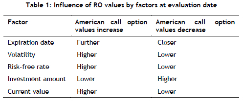
The first row of Table 1 shows that the call option value increases at the evaluation date when the expiration date is far away from the RO evaluation date; and the inverse occurs. The investment amount is the only factor that moves in the opposite direction to the call option values. The influence of factors in Table 1 is easily observed when two or more ROs are evaluated at the same evaluation date.

1.2. Sequential compound real options applications

The sequential compound real options (SCROs) are where later ROs become available, but only if the earlier one is exercised [21]. In [9], the SCROs are defined as ROs when the second is created, but only if the first is exercised. The SCROs were introduced in [20] without a model. A model was developed in [21], based on a continuous time interval. In [9], a model for evaluating the SCROs based on a discrete time interval was introduced.

In [10], the SCRO model was applied to a research and development (R&D) manufacturing investment opportunity that had four sequential investment opportunities. In [11], the SCRO model was applied when evaluating an investment project, which expanded after two years; after a further two years, half of the project was sold. In [22], the SCRO model was applied to a new chemical plant, where the decision-makers needed to know whether they should commit to investing the total amount needed, or defer, or abandon the investment. In [23], the SCRO model was adjusted and applied to an oil production project.

The present authors were not able to find any literature with SCRO applications in South Africa. However, RO models were used for capacity expansion in the construction material industry [24], in physical asset management capital budgeting investments [25], and in cellular telecommunication capital investments [26]. A survey in [18] showed that about 11% of South African companies were using the RO models in 2008.

The literature review discussed above shows that SCROs have been applied to construction projects, R&D manufacturing investments, and oil projects, but not to electricity expansion projects. The questions that this study is attempting to answer are:

• Can the SCRO be evaluated a step-by-step approach?

• What is the outcome of applying the SCRO in the case of South African electricity capacity expansion, considering the FBCwCCS investment project?

The remainder of this study covers the development of the SRCO method in section 2; the NPV background and applications in section 3; the data used for the application of the SCRO in section 4; applications of the SCRO method in section 5; the results in section 6; the study discussion in section 7; and the conclusion in section 8. Appendix A discuss the inflation simulation, and the call option values for the second and first investment projects are in appendices B and C, respectively.

 

2. THREE-STEP METHOD FOR SEQUENTIAL COMPOUND REAL OPTION EVALUATION

This study developed the SCRO evaluation method from the application in [22]. The SCRO method is divided into three steps: a determination of the RO factors, a determination of the gross project value, and a determination of the American call options.

2.1. Step 1: Determination of the RO factors

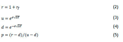
The RO factors σ,u, d, and ρ are determined. Volatility, σ, is a standard deviation of historical returns, rj [22]. It is assumed that historical revenues less operating costs (H) follow a lognormal distribution [23]. The values of rj, are derived from equation (1) [23].

In equation (1) the years are represented by In equation (2) rf is the risk free rate. In equations (3) and (4) σ is used to determine u and d respectively, and ΔT is the time frequency [9]. In equation (4) ρ is a risk-free probability [23].

2.2. Step 2: Determining gross project value

The value of the initial gross project, V₀, is determined by equation (6).

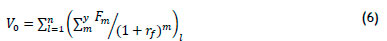
In equation (6), F is the expected cash flow, m is the number of years from the cash flow year to the evaluation date [27], I is the number of investment projects. Equation (6) is the sum of the η investment present values, where the term inside the brackets is a present value formula [27].

The value of V₀, goes up by a factor of u and down by d each year until the last investment year [9], which is z. The up and down movements of V₀ form a binomial tree [9], [22], which is in Table 2 for the first three years. The binomial tree is used because it embodies the uncertainty associated with each V₀ [10]. The values of V₀ are not constant, but are to be adjusted as new information emerges [10].

 

 

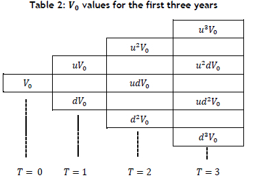
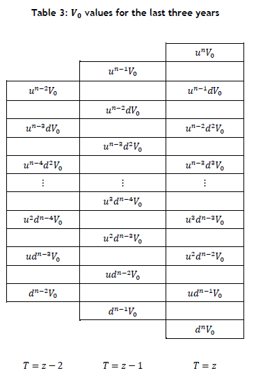
It is important to note that, in Table 2, the order of ups and downs does not matter. As an example: dududV₀ = uudddV₀ = ddduuV₀ = d³u²V₀. Table 3 shows the last three years, z - 2, z - 1 and z of the binomial tree.

 

 

2.2.1. SCRO values for the investment at Τ = Z

In this step, decisions are made about the I investment projects, starting with the investment project that expires at Τ = z. The call option values at Τ = z are represented by Ci_l,z, which corresponds to the investment cost /_i, and are derived from equation (7) [9].

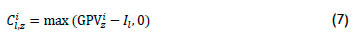
In equation (7), i represents the number of rows in each column of Table 3; for example, for Τ = z, i = 1, -, z + 1. The call options values at Τ = z are used to determine call option values at Τ = z - 1, where ϊ' = 1, ..., z, using equation (8) [10].

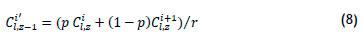
Equation (8) is used to determine the call option values at Τ = z - 1. Similarly, the call option values at Τ = z - 2 are determined from the call option values at Τ = z - 1. The determination of call option values from the previous year's call option values continues until Τ = 0.

2.2.2. SCRO values for the investment at Τ = z-1

The call option values for the investment project cost, are determined from the resultant binomial tree in section 2.2.1. The call option values at Τ = z - 1, is c^j_l__1z-1, where j = 1, ... ,z, are determined from equation (9).

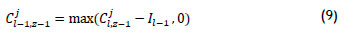
Similar to equation (8), equation (10) is used to determine the call option values at Τ = ζ - 2, which are determined from the call option values at Τ = z - 1. In equation (10), j' = 1, -,z - 1.

Similar to section 2.2.1, the call option values determined in this section result in a binomial tree.

2.2.3. SCRO values for the investment at Τ = z-2

The call option values for, i_l_₂, are determined from the call option values in section 2.2.2. However, only the call option values at Τ = z - 2 are considered, because this is when I_l_₂ is invested. The call option values for I_l_₂ at Τ = z - 2 are determined from equation (11), where k = 1, -, z - 1.

 

Similar to sections 2.2.1 and 2.2.2, the call option values at Τ = z - 3 are derived from the call option values at Τ = z - 2, as shown in equation (12), where k' = 1, -,z - 2.

The call options determined in equation (12) are used to determine the call at Τ = z - 3,z-4, - ,0. The call option value for this investment at Τ = 0 is used to determine whether the total investment for the I projects should be invested or deferred.

2.3. Data required for SCRO method

The SCRO method requires the following data for each investment project: evaluation date, investment date, investment amounts, and expected cash flows. Economic and additional data is required to determine the factors discussed in section 2.1.

 

3. NET PRESENT VALUE: BACKGROUND

The NPV was introduced in the 19^th century by engineers for comparing investment proposals, and was adopted by economists in the 20^th century [28]. The NPV is defined as a traditional approach to evaluating potential capital investment projects [6]. It is a discounted cash flow criterion for comparing future capital investment projects [3]. The NPV is used in decision-making by businesses [29]. The determination of the NPV requires both the discount rate and the cash flows. The NPV is given by equation (13) [7].

In equation (13), CF₀ is the initial investment with a negative sign. There can be negative cash flows other than CF₀ when there are several investments at different periods. In equation (13), y is a period when the cash flow occurred relative to the NPV evaluation date; s is a discount rate. The NPV results are interpreted as follows [8]: if the NPV is less than zero, the investor is better off without the investment; and if it is greater than zero, the investor is better off with the investment.

3.1. Applications of the NPV method

The applications of the NPV method discussed in this subsection focus on two aspects. The first aspect is about further developments in the NPV formula in equation (13), and the second is about the actual application of the NPV method by companies.

In [30], it is acknowledged that the cash flows in equation (13) are usually uncertain. As a result, a new method based on scenario planning and the decision-maker's attitude is proposed in [30].

As mentioned in section 2.3, equation (13) can be used in cases where there are several investments during the life of the project. In [31], such cases are referred to as non-conventional cashflows. The NPV is not appropriate for evaluating investment projects with non-conventional cashflows [31], [32]. However, equation (6) shows that the SCRO method can evaluate such projects.

Equation (13) requires the value of s, which is usually determined from the capital costs of a company, which requires some guesswork [29]. According to [29], there are also no rules for determining the value of s. The downside of s can also be inherited by the Ro through equation (6), which is a sum of present values. The SCRO or RO formula is an extension of the NPV [8]. In [12], the value of the RO is expressed as the sum of the NPV and the strategic value. However, at the RO expiration date the NPV and RO values of a project are the same [33].

The applications of the NPV method by companies do not provide the details of which NPV method is used, but surveys have determined whether or not the companies have used the method. The 2006 survey showed that 82% of South African companies used the NPV method [34]. The larger South African companies used the NPV method together with other methods, whereas smaller companies did not use the NPV method at all [34]. However, the survey in [26] showed that the NPV method was not the method preferred by South African state-owned companies for capital budgeting. The delay in adopting the NPV method is attributed to the time lag between theory and implementation [26], [34]. There might also be other reasons for not using the NPV method, other than the time lag, because it was introduced in the late 1800s to early 1900s [25].

 

4. FBCWCCS TECHNOLOGY AND ECONOMIC DATA

The FBCwCCS technology data used in this study is from the two-stage stochastic linear programming (TSSLP) study in [1], which was extended by changing the TSSLP to the two-stage stochastic mixed integer linear programming (TSSMILP) model. The data in Table 4 is extracted from the TSSMILP results.

 

 

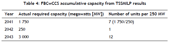
The first row of Table 4 shows that the power plant with seven units was to be in operation in 2041, the second with one unit in 2042, and the third with 12 units in 2043. The second power plant can be added to the first or the third power plant. However, in this study it is analysed as a stand-alone power plant.

4.1. FBCwCCS expected cash flows

The FBCwCCS investment projects do not have underlying values like financial investments [15]. As discussed in section 2.2, the expected cash flows are used to determine . There is no data for expected cash flows, f_t; as a result they are determined from equation (14).

In equation (14), t is the time period for each cash flow; v_t is the revenue in year t; g_t is the corresponding running costs i.e. fuel and fixed and variable operation and maintenance (O&M) costs.

In equation (15), q_t represents the electricity generated at time t, p_t is the electricity price, and x_t is a quotient of electricity sold to electricity generated. The historical average value of x_t from 2009/10 to 2019/20 is 89% [35]. The values of x_t are used to simulate future values, based on Chebyshev's theorem [36] because of future uncertainty. Based on the theory in [36], it is assumed that the future values of x_t move randomly between two standard deviations above and below the historical average, and this assumption accommodates 95% of the future values; the other 5% lies outside the two standard deviation boundaries.

The random values for each investment project for each year are determined in MS Excel using the RANDBETWEEN function in [37]. The average of 500 simulations is then used to determine the revenue for each investment project, for each [38].

The value of p_t is 86.35 c/kWh, which is derived from Eskom's total electricity sales of 208.32 terawatt hours and the revenue of R180 billion for t = 2020 [35]. However, where t > 2020, p_t is adjusted by the corresponding annual inflation, as shown in Figure 1.

 

 

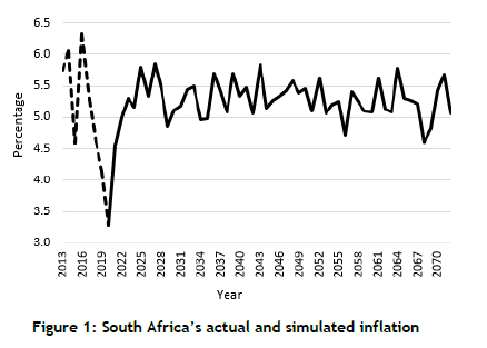
In Figure 1 the annual inflation rates from 2013 to 2020 (dotted line) are actual and the rest are simulated. The determination of the simulated annual inflation rates is discussed in Appendix A.

The resultant cash flows for the FCBwCCS investment projects are derived from equation (14) and are shown in Figure 2. The resultant cash flows are increased by the corresponding inflation rate because Eskom's value of p_t is expected to increase. The cash flows in Figure 2(a) show that t starts from 2041 and goes to 2070. The cash flows in Figure 2(a)-(c) are used to determine the V₀.

 

 

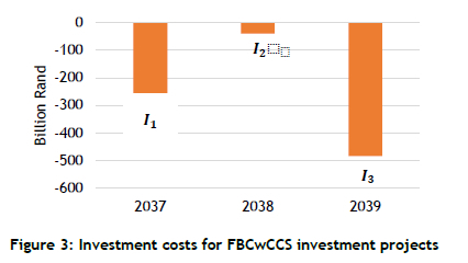
4.2. FBCwCCS investment costs

The investment costs in Figure 3 are determined as at 2013 in the TSSMILP model, and are adjusted by the inflation rates in Figure 1, from 2013 to the respective years shown in Figure 3. I₁, I₂, and I₃ have option durations of 17 years (2020 to 2037), one year (2037 to 2038), and one year (2038 to 2039) respectively. The resultant investment costs are I₁= R254.54 billion, I₂= R38.04 billion, and I₃= R489.19 billion.

 

 

4.3. South African economic data

Economic data is required for the SCRO evaluation. The value of r_f is the difference between the South African 30-year bond yield as of 31 December 2020 of 10.797% [39] and the corresponding inflation rate of 3.3% [40].

 

5. SCRO METHOD APPLIED TO FBCWCCS INVESTMENT PR0JECTS

The method developed in section 2 and the data discussed in section 3 are used to evaluate the FBCwCCS investment projects. The differences between the application in [22] and this paper are that:

• In [22] a new chemical plant is evaluated, whereas this study is based on power plants.

• In this study, uncertainty is in future cash flows, which are influenced by uncertain electricity demand and are quantified and discussed in section 3.1.1.

• In this study, three new power plants are based on the same technology, FBCwCCS, and are assumed to derive revenue from the same market. Thus the same volatility is used.

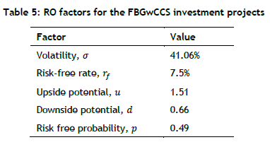
5.1. Step 1: Determination of RO factors

The factors are determined from the formulae in section 2.1 and the data in section 3. The factor results are in Table 5.

 

 

5.2. Step 2: The V₀ determination for FBCwCCS investment projects

Table 6 presents the value of V₀ at Τ = 2020, which is determined from equation (6) and the cash flows in Figure 2. The value of rf is from Table 5 and η = 3 because the FBCwCCS has three successive investments. For the first investment project, the cash flows are from m = 2041 to 2070, from 2042 to 2071 and from 2043 to 2072 for the second and third investment projects, respectively. The values of in equation (6) are from 1,...,30 for all of the investment projects.

 

 

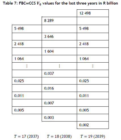
In Table 6 the value of V₀ is R5.11 billion at Τ = 0, and increases to R7.71 by a factor of u or decreases to R3.39 billion by a factor of d at Τ = 1; this continues until Τ = 3. However, Table 7 shows the values of V₀ for the last three years in which the three investment projects are invested (2037, 2038, and 2039).

 

 

5.3. Step 3: Determination of the SCRO values

The SCRO values are determined from the values of V₀ in section 4.2. In this step, decisions are made about the three investment projects, starting at Τ = 19.

5.3.1. SCRO values for investment at Τ = 19

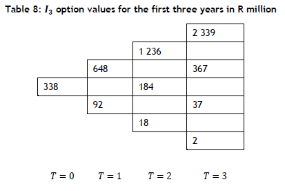
The call options, C₃₁₉, correspond to investment cost I₃ at Τ = 19, and are derived from equation (7) in section 2.2.1 and shown in equation (16).

Equation (7) is used for all values of i until i = z + 1 = 20, where C²⁰_3,19 = 0. The call options values at Τ = 19 are used to determine the call option values at Τ = 18, where i' = 1, ... ,19, using equation (17), which is based on equation (8).

Equation (8) is used to determine all of the call options values at = 18. Similarly, the call option values at Τ =17 are determined from the call option values at Τ = 18. The determination of call option values from the previous year's call option values continue until = 0. The resultant binomial trees are shown in Table 8 for the first three years and in Table 9 for the last three years.

 

 

 

 

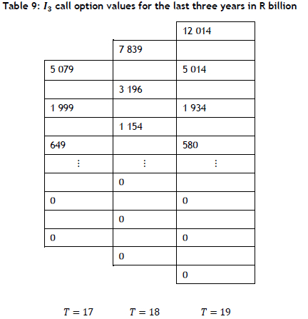
5.3.2. SCRO values for investment at Τ = 18

The call option values for I₂ are determined from the call option values C^j_3,18, in Table 9 at Τ = 18, which corresponds to this investment year for this project and = 1, ... ,19. The call option values at Τ =18 are determined from equation (10) which results in equation (18).

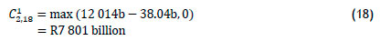
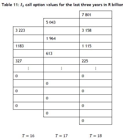
Using equation (10), the results for the rest of the call options at Τ = 18 are: C²_2,18 = R3 158, C³₂,₁₈ = R1 115. and C⁴_2,18 = R225 billion, and the rest of the call option values are equal to zero. As shown before, the call option values at Τ = 18 form the first column of Table 11 in appendix B. Similarly, the call option values at Τ = 17 are determined from the call option values at Τ = 18 using equation (11). The resultant call option values are C₂¹₁₇ = R5 043, C₂²₁₇ = R1 964, C₂³₁₇ = R613, and C2*₁₇ = R102 billion, and the rest are equal to zero. The call option values at Τ = 16 are determined from the call option values at Τ = 17; this carries on until Τ = 0. These option values form the binomial trees in Appendix B.

5.3.3. SCRO values for investment at Τ = 17

The call option values corresponding to the investment I₁ are determined from the I₂ call option values determined in section 4.3.2. However, only the call option values at Τ = 17 (2037) are considered because this is when I₁ is invested. The call option values for I₁ at Τ = 17 are determined from equation (11), where k = 1, as shown in equation (19).

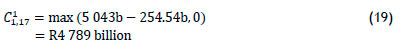
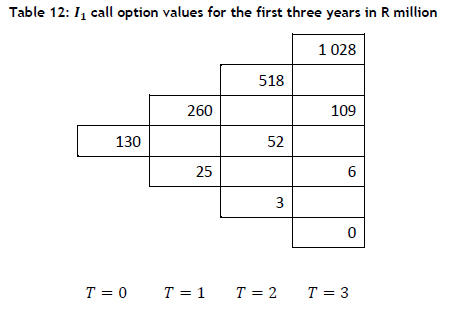
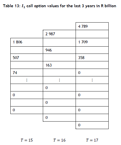
For k = 2, ... ,18 the call option values determined from equation (11) and are C²_1,17 = R1 709 and C³_1,17 = R358 billion, and the rest are equal to zero. Similar to sections 4.3.1 and 4.3.2, the call option values at Τ = 16 are derived from the call option values at Τ =17 using equation (13). Their values are C¹_1,16 = R2 987, C²_1,16 = R946, and C³_1,16 = R163 billion, and the rest are equal to zero. The call option values at T=15 are determined from the call option values at Τ = 16; this carries on until Τ = 0. The call option values results are in Table 12 and Table 13 in appendix C.

 

6. RESULTS

The results for the FBCwCCS investment projects are discussed, based on the SCRO method and the NPV approach.

6.1. SCRO results

The call option value determined in section 4.3.3 at Τ = 0 for I₁ is R130 million, as shown in Table 12 in Appendix C, and is used to decide whether or not to exercise the option of investing in FBCwCCS projects. If the start-up costs are less than or equal to R130 million, decision-makers are advised to invest in these projects, or otherwise to defer the investments. This first investment has an option duration of 17 years, which is long enough for the option value of R130 million to grow in favourable economic conditions.

6.2. NPV results

The NPV for the three investment projects is determined from equation (13), using the cash flows determined in section 3.1 and the investment costs determined in section 3.2. In equation (13) s is the discount rate; however, r from equation (2) and the value of ry in Table 5 are used. The valuation date is 2020, but the cash flows are in Figure 2 and the investment costs are in Figure 3. The combined NPV for the three investments is -R202 billion. The negative NPV means that the FBCwCCS investment projects should not be considered.

 

7. DISCUSSION

The real option results in this paper provide decision-makers with the option to exercise the investment or to defer it until the value of the underlying asset is more than the start-up costs. However, the NPV results suggest that the investments should not be considered. As mentioned in section 2.3.1, there is a relationship between the RO and the NPV. Nonetheless, there is a deviation between the RO and NPV results for the FBCwCCS investment because this investment has an option duration of 17 years. When the option duration decreases, the RO and NPV results converge [33].

Low revenues contribute to the value of the underlying assets for the RO. Revenues are low because of the low value of p_t. The value of p_t is affected by Eskom's historical revenues and total sales, which in turn are affected negatively by customers who are not paying for electricity [41]. The South African electricity price is also not cost-reflective [42]. Even though South Africa has experienced high electricity increases, the electricity price is still 40% less than those in other countries [41].

Volatility is assumed to be constant throughout the power plants' economic lives. In reality, volatility will change and influence the call option values, as indicated in Table 1.

One should also bear in mind that the data used in this paper is taken from a mixed integer linear two-stage stochastic programming model's results. The simulated inflation rates are used to increase the technology costs, and are too conservative when compared with the actual technology cost increases.

South African companies are lagging behind in the use of the NPV when compared with companies in the USA, the UK, and Australia [34]. The same pattern is observed in the use of RO, where companies in the USA, the UK, the Netherlands, Germany, and France have increased the use of RO from 26% to 53%. By contrast, the use of RO by South African companies is way below 20% [34].

 

8. CONCLUSION

In this study, a three-step sequential compound real options (SCRO) method is developed and applied to FCBwCCS investment projects. The SCRO method is used and compared with the traditional net present value (NPV) method. Electricity demand is considered as the source of uncertainty, and is quantified by assuming a random movement of the quotient of electricity revenue to electricity sold.

The SCRO results based on the South African FCBwCCS investment projects show that decision-makers can exercise the option to invest if the initial costs are less than or equal to R130 million, or otherwise defer the investments. The call option to defer enables real option value to grow during the remaining duration of the call option. The NPV results show that investors are better off without the FCBwCCS investment projects.

The NPV is a popular method for investment evaluation when compared with the RO method. The NPV has its shortcomings, which are discussed in the literature; hence the SCRO method. However, the results of the two methods diverge when the call option duration is long, which is the case in this study.

Even though there is development in the RO literature, there is a slow intake of such new methods by the industry. Nevertheless, developed countries show growth in their use of the RO, which will ultimately filter down to countries like South Africa. The NPV has followed a similar pattern.

 

REFERENCES

[1] M. Bashe, M. Shuma-Iwisi and A. M. van Wyk, "Application of stochastic programming to the electricity generation planning in South Africa," Orion, vol. 35, pp. 88-125, 2019.         [ Links ]

[2] South African Department of Energy, "Integrated resource plan for electricity 2010-2030 update report," 2013. [Online]. Available: https://www.environment.gov.za/sites/default/files/docs/irp2010_2030.pdf [Accessed 28 June 2019].         [ Links ]

[3] South African Department of Energy, "Request for comments: Draft integrated resource plan 2018," 2019. [Online]. Available: http://www.energy.gov.za/IRP/irp-update-draft-report2018/IRP-Update-2018-Draft-for-Comments.pdf [Accessed 22 October 2019].         [ Links ]

[4] South African Department of Energy, "Integrated resource plan for electricity 2010-2030 Final Report," 2011. [Online]. Available: http://www.energy.gov.za/IRP/irpfiles/IRP2010_2030_Final_Report_20110325.pdf [Accessed 15 July 2019].         [ Links ]

[5] South African Department of Energy, "Integrated resources plan 2019," 2019. [Online]. Available: http://www.energy.gov.za/IRP/2019/IRP-2019.pdf [Accessed 2 February 2021].         [ Links ]

[6] C. J. Hull, Options, futures and other derivatives, 6th ed. Boston Prentice Hall, 2005. J. Fernando, "Net present value (NPV)," 2021. [Online]. Available: https://www.investopedia.com/terms/n/npv.asp [Accessed 8 December 2021].         [ Links ]

[7] T. A. Luehrman, "Investment opportunities as real options: Getting started on the numbers," Harvard Business Review, vol. 76, no. 4, pp. 51-67, 1998.         [ Links ]

[8] T. Copeland and V. Antikarov, Real options: A practitioner's guide, Knutsford: Texere, 2001.         [ Links ]

[9] H. S. B. Herath and C. S. Park, "Multi-stage capital investments opportunities as compound real options," The Engineering Economist, vol. 47, no. 1, pp. 1-27, 2002.         [ Links ]

[10] T. Radjenovic, "Real options," Series of Economics and Organization, vol. 5, no. 1, pp. 83 -92, 2003.         [ Links ]

[11] V. Csapi, "Applying real options theory in the electric energy sector," Public Finance Quaterly, State Audit Office of Hungary, vol. 58, no. 4, pp. 469-483, 2013.         [ Links ]

[12] T. A. Luehrman, "Strategy as a portfolio of real options," Harvard Business Review, vol. 76, no. 5, pp. 89-99, 1998.         [ Links ]

[13] L. Trigeorgis, "Real options and investment under uncertainty: What do we know?" 2002. [Online]. Available: https://ideas.repec.org/p/nbb/reswpp/200205-3.html [Accessed 7 December 2019].         [ Links ]

[14] J. C. Hull, Options, futures and other derivatives, 6th ed. Boston Prentice Hall, 2005.         [ Links ]

[15] Y. Zhang, "An analysis and comparison of real option approaches for project valuation under uncertainty," Masters diss. University of Otago, 2010.         [ Links ]

[16] R. Brosch, Portfolios of real options. Lecture notes in economics and mathematical systems, vol. 611, Berlin Springer, 2008.         [ Links ]

[17] J. C. Hull, Options, futures and other derivatives, 8th ed. Boston Prentice Hall, 2012.         [ Links ]

[18] V. Csapi, "How real option theory has gained space in research and practice - An overview of the last four decades," International Research Journal of Finance and Economics, vol. 171, pp. 86-95, 2019.         [ Links ]

[19] F. Black and M. Scholes, "The pricing of options and corporate liabilities," Political Economy, vol. 81, no. 3, pp. 637-654, 1973.         [ Links ]

[20] R. Geske, "The valuation of compound options," Financial Economics, vol. 7, pp. 63-81, 1979.         [ Links ]

[21] T. Copeland and P. Tufano, "A real world way to manage real options," Harvard Business Review, vol. 82, pp. 91-99, 2004.         [ Links ]

[22] L. E. Brandao, J. S. Dyer and W. J. Hahn, "Using binomial decision trees to solve real-option valuation problem," Decision Analysis, vol. 2, no. 2, pp. 69-88, 2005.         [ Links ]

[23] A. M. Momani, T. H. Al-Hawari and R. W. Mousa, "Using expanded real options analysis to evaluate capacity expansion decisions," South African Journal of Industrial Engineering, vol. 27, pp. 1-14, 2016.         [ Links ]

[24] C. A. Campher, "Exploring real options in the capital budgeting of investments within physical asset management," Masters diss. Stellenbosch University, 2012.         [ Links ]

[25] M. Mkhize and N. Moja, "The application of real option valuation techniques in the cellular telecommunication industry in South Africa," South African Journal of Business Management, vol. 40, pp. 1-20, 2009.         [ Links ]

[26] CFI Team, "Time value of money," [Online]. Available: https://corporatefinanceinstitute.com/resources/knowledge/valuation/time-value-of-money/ [Accessed 20 February 2021].         [ Links ]

[27] T. W. Jones and J. D. Smith, "An historical perspective of net present value and equivalent annual cost," The Accounting Historians Journal, vol. 9, pp. 103-110, 1982.         [ Links ]

[28] S. Le, "The applications of NPV in different types of markets," in Proceedings of the 2021 3rd International Conference on Economic Management and Cultural Industry. [Online]. Available: https://www.atlantis-press.com/proceedings/icemci-21/125966042 [Accessed 13 February 2021].         [ Links ]

[29] H. Gaspars-Wieloch, "Project net present value estimation under uncertainty," Central European Journal of Operations Research, vol. 27, pp. 179-197, 2019.         [ Links ]

[30] M. Illes, "The positive net present value of loss making projects: Economic content of two internal rates of return," Journal of Economic Literature, vol. 16, pp. 41-50, 2020.         [ Links ]

[31] O. Erdem, T. Guyagule and N. Demirel, "Uncertainty assessment for the evaluation of net present value: A mining industry perspective," The Journal of The Southern African Institute of Mining and Metallurgy, vol. 112, no. 5, pp. 405-412, 2012.         [ Links ]

[32] T. A. Leuhrman, "Investment opportunities as real options: Getting started on the numbers," Harvard Business Review, vol. 76, no. 4, pp. 51-67, 1998.         [ Links ]

[33] C. Correia, "Capital budgeting practices in South Africa: A review," South African Journal of Business Management, vol. 43, pp. 11-29, 2012.         [ Links ]

[34] Eskom, "Integrated report," March 2020. [Online]. Available: https://www.eskom.co.za/IR2020/Pages/default [Accessed 2 January 2020].         [ Links ]

[35] T. A. Ferryman and S. K. Cooley, "Data outlier detection using the Chebyshev theorem," in IEEE Aerospace Conference Proceedings, pp. 3814-3819, 2005.         [ Links ]

[36] G. Ulrich and L. T. Watson, "A method for computer generation of variates from arbitrary continuous distributions," SIAM Journal of Scientific Computing, vol. 2, no. 2, pp. 185-197, 1987.         [ Links ]

[37] T. Kennedy, "Monte Carlo methods - A special topics course," 27 April 2016. [Online]. Available: https://www.math.arizona.edu/-tgk/mc/book.pdf [Accessed 15 May 2021].         [ Links ]

[38] World Government Bonds, "South Africa government bonds - Yields curve,"2 May 2021, [Online]. Available: http://www.worldgovernmentbonds.com/bond-historical-data/southafrica/ [Accessed 2 May 2021].         [ Links ]

[39] STATSSA, "Consumer price index December 2020," 2020. [Online]. Available: http://www.statssa.gov.za/publications/P0141/P0141December2020.pdf [Accessed 15 March 2021].         [ Links ]

[40] Staff Writer, "Electricity prices in South Africa vs the world," 3 July 2020. [Online]. Available: https://mybroadband.co.za/news/energy/358277-electricity-prices-in-south-africa-vs-the-world.html [Accessed 29 May 2021].         [ Links ]

[41] Eskom, "Strategic direction and tariff design principles for Eskom's tariffs 2017," 2017. [Online]. Available: http://www.eskom.co.za/CustomerCare/TariffsAndCharges/Documents/Strategicpricingdirection201725-07-2017.pdf [Accessed 9 October 2019].         [ Links ]

[42] STATSSA, "Consumer price index October 2019," 20 November 2019. [Online]. Available: http://www.statssa.gov.za/publications/P0141/P0141October2019.pdf [Accessed 25 November 2019].         [ Links ]

[43] STATSSA, "Consumer price index November 2019," 11 December 2019. [Online]. Available: http://www.statssa.gov.za/publications/P0141/P0141November2019.pdf [Accessed 12 December 2019].         [ Links ]

[44] STATSSA, "Gross domestic product fourth quarter 2019," March 2020. [Online]. Available: http://www.statssa.gov.za/publications/P0441/P04414thQuarter2019.pdf [Accessed 14 May 2021].         [ Links ]

[45] STATSSA, "Gross domestic product fourth quarter 2020," March 2021. [Online]. Available: http://www.statssa.gov.za/publications/P0441/P04414thQuarter2020.pdf [Accessed 14 May 2021].         [ Links ]

[46] South African Reserve Bank, "Monetary policy," [Online]. Available: https://www.resbank.co.za/en/home/what-we-do/monetary-policy [Accessed 19 April 2021].         [ Links ]

[47] D. Aydin and B. Senoglu, "Monte Carlo comparison of the parameter estimation methods for the two-parameter Gumbel distribution," Journal of Modern Applied Statistical Methods, vol. 14, no. 2, pp. 123-140, 2015.         [ Links ]

[48] Eskom, "Eskom integrated report," 2019. [Online]. Available: http://www.eskom.co.za/IR2019/Documents/Eskom_2019_integrated_report.pdf [Accessed 1 September 2019].         [ Links ]

[49] S. Riederova and K. Ruzickova, "Historical development of derivatives' underlying assets," Acta Universitatis Agriculturae et Silviculturae Mendelianae Brunensis, vol. 59, no. 7, pp. 521-526, 2011.         [ Links ]

[50] S. C. Myers, "Determinants of corporate borrowing," Financial Economics, vol. 5, pp. 147-175, 1977.         [ Links ]

[51] L. Trigeorgis, Real options: Managerial flexibility and strategy in resource allocation. London, The MIT Press, 1996.         [ Links ]

[52] N. Georgiopoulos, "Real options: an introduction with applications," Masters diss. 2004. [Online].         [ Links ]

[53] W. T. Lin, C. F. Lee and C. W. Duan, "Multistage compound real options: Theory and application," in Encyclopedia of Finance, Springer, 2006.         [ Links ]

[54] P. Kodukula and C. Papudesu, Project valuation using real options: A practitioner's guide, Fort Lauderdale, J. Ross Publishing, 2006.         [ Links ]

[55] Eskom, "Connect: The 2019/20 Nersa-approved price increase," [Online]. Available: http://www.eskom.co.za/CustomerCare/TariffsAndCharges/Documents/Connect2019_20.pdf [Accessed 21 September 2019].         [ Links ]

[56] South African Reserve Bank, "The inflation target," [Online]. Available: https://www.resbank.co.za/MonetaryPolicy/DecisionMaking/Pages/InflationMeasures.aspx [Accessed September 2019].         [ Links ]

[57] National Treasury Republic of South Africa, "Budget review," 2019. [Online]. Available: http://www.treasury.gov.za/documents/nationalbudget/2019/review/FullBR.pdf [Accessed 1 September 2019].         [ Links ]

[58] National Energy Regulator of South Africa, "Monitoring renewable energy performance of power plants," [Online]. Available: http://www.nersa.org.za/Admin/Document/Editor/file/Electricity/SustainableEnergy/MonitoringRenewablePerformanceofPowerPlants-Trackingprogressof2017-Issue11(March2018).pdf [Accessed 12 August 2019].         [ Links ]

[59] Eskom, "Eskom revenue application - Multi-year price determination (MYPD 4) FY2019/20 - 2021/22," September 2018. [Online]. Available: http://www.nersa.org.za/Admin/Document/Editor/file/Consultations/Electricity/Notices/EskomSummaryMYPD4.pdf [Accessed 17 November 2019].         [ Links ]

[60] EPRI, "Power generation technology data for integrated resource plan of South Africa," August 2015. [Online]. Available: http://www.energy.gov.za/IRP/2016/IRP-AnnexureA-EPRI-Report-Power-Generation-Technology-Data-for-IRP-of-SA.pdf [Accessed 9 October 2019].         [ Links ]

[61] EPRI, "Power generation technology data for integrated resource plan of South Africa," April 2017. [Online]. Available: http://www.energy.gov.za/IRP/irp-update-draft-report2018/EPRI-Report-2017.pdf [Accessed 10 October 2019].         [ Links ]

[62] Eskom, "Eskom integrated report," 2017. [Online]. Available: http://www.eskom.co.za/IR2017/Pages/default.aspx [Accessed 17 March 2019].         [ Links ]

[63] Eskom, "Eskom integrated report," 2018. [Online]. Available: http://www.eskom.co.za/IR2018/Documents/Eskom2018IntegratedReport.pdf [Accessed 1 September 2019].         [ Links ]

[64] J. Mun, Real options analysis: Tools and techniques for valuing strategic investments and decisions, Haboken Wiley & Sons, 2002.         [ Links ]

[65] National Energy Regulator of South Africa, "Monitoring renewable energy performance of power plants," [Online]. Available: RenewablePerformanceofPowerPlants-Trackingprogressof2017-Issue11(March2018).pdf [Accessed 12 August 2019].         [ Links ]

[66] World Government Bonds, "South Africa government bonds," 2 August 2019. [Online]. Available: http://www.worldgovernmentbonds.com/country/south-africa/ [Accessed 2 August 2019].         [ Links ]

[67] A. K. Dixit and R. S. Pindyck, Investment under uncertainty, Princeton, Princeton University Press, 1994.         [ Links ]

[68] Eskom, "Tariffs and charges," 2019-2020. [Online]. Available: https://www.eskom.co.za/CustomerCare/TariffsAndCharges/Documents/CompleteTariff2019web1.pdf [Accessed 28 November 2019].         [ Links ]

[69] S. Kadry, "Monte Carlo simulation using Excel: Case study in financial forecasting," in The Palgrave Handbook of Research Design in Business and Management. New York, Palgrave Macmillan, 2015, pp. 263-289.         [ Links ]

[70] D. G. Altman and J. M. Bland, "Standard deviations and standard errors," BJM, vol. 331, p. 903, 2005.         [ Links ]

[71] Statista, "Global electricity prices in 2018 by selected country," 2019. [Online]. Available: https://www.statista.com/statistics/263492/electricity-prices-in-selected-countries/ [Accessed 14 December 2019].         [ Links ]

[72] STATSSA, "Consumer price index January 2015," 18 February 2015. [Online]. Available: http://www.statssa.gov.za/publications/P0141/P0141January2015.pdf [Accessed 19 November 2019].         [ Links ]

[73] STATSSA, "Consumer price index June 2011," 20 July 2011. [Online]. Available: http://www.statssa.gov.za/publications/P0141/P0141June2011.pdf [Accessed 20 November 2019].         [ Links ]

[74] D. Aydin and B. Senoglu, "Monte Carlo comparison of the two parameter estimation," Journal of Mordern Applied Statistical Methods, vol. 14, pp. 123-140, 2015.         [ Links ]

[75] Eskom, "Integrated results," March 2020. [Online]. Available: https://www.eskom.co.za/IR2020/Pages/default.aspx [Accesssed 15 April 2021].         [ Links ]

[76] T. Mutshutshu, "Capital budgeting techniques employed by selected South African state-owned companies," 2013. [Online]. Available: https://repository.up.ac.za/handle/2263/42895Prince [Accessed 30 June 2022].         [ Links ]

 

 

Accepted for publication 21 Mar 2023
Available online 26 May 2023
Submitted by authors 16 Dec 2021

 

 

* Corresponding author: mbashe@mweb.co.za
ORCID® identifiers
M. Bashe: https://orcid.org/0000-0001-7192-8189
M. Shuma-Iwisi: https://orcid.org/0000-0002-8879-2369
M.A. van Wyk: https://orcid.org/0000-0002-4519-1475

 

 

APPENDIX A

This appendix discusses how the South African inflation rates are simulated. The historical year-on-year inflation rates (Η) from January 2009 to December 2020 are taken from Statistics South Africa's reports [43], [44], [45], [46]. Year 2009 is chosen because it was when South Africa started to target the year-on-year inflation rates to fall between 3% and 6% [47].

The distribution of the historical Η is determined from R software [37]. The inverse distribution, Y = F^-1(U), is used to simulate year-on-year inflation rates from 2021 to 2072, where U is a random uniform variate generated by function RAND() in MS Excel [48]. The results are shown in Figure 1.

 

APPENDIX B

The call option values in Table 10 and Table 11 are for the I₂, and are determined in section 2.2.2.

 

 

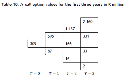
The option values at Τ = 18 are determined first from equation (10). Equation (11) is used to determine the call option values at Τ = 17, based on the Τ = 18 call option values; this continues iteratively until Τ = 0.

 

 

APPENDIX C

The call option values for I₁ are determined from the call option values in appendix B at Τ =17 using equation (12). The option values at Τ = 16 are determined from the option values at Τ = 17 using equation (13). Similarly, the call option values at Τ = 15 are determined from the call option values at Τ = 16, and this continues iteratively until Τ = 0. The results are shown in Table 12 and Table 13.