GENERAL ARTICLES

 

A machine-learning approach towards solving the invoice payment prediction problem

 

 

L. Schoonbee; W.R. Moore; J.H. van Vuuren^*

Department of Industrial Engineering, Stellenbosch University, South Africa

 

 

---

ABSTRACT

Companies routinely experience difficulties in collecting debt incurred by their customers. As an alternative to the reactive techniques typically employed to increase a company's ability to collect debt, preventative techniques could be employed to predict the payment behaviour of regular customers. Such a preventative technique, in the form of a machine-learning model embedded within a decision-support system, is proposed in this paper with a view to assisting companies in prioritising debt collection resources to address invoices that are most likely to be paid late. The system is capable of predicting payment behaviour outcomes linked to invoices as anticipating payment receipts during one of three intervals: 1-30 days late, 31-60 days late, or at least 61 days late. The underlying model of the decision support system is identified by selecting a suitable algorithm from among a pool of candidate machine-learning algorithms. This selection process requires the adoption of a sound methodological approach. A machine-learning development roadmap is proposed for this purpose, and applied in a practical, illustrative case study involving real industry invoice data.

---

OPSOMMING

Maatskappye ondervind dikwels probleme met die invordering van skuld wat deur hul kliënte aangegaan word. As 'n alternatief tot reaktiewe tegnieke wat tradisioneel toegepas word om 'n maatskappy se vermoë om skuld in te vorder, te verhoog, kan voorkomende tegnieke aangewend word om die betalingsgedrag van gereëlde kliënte te voorspel. So 'n voorkomende tegniek, in die vorm van 'n masjienleermodel wat in 'n besluitsteunstelsel ingebed is, word in hierdie artikel voorgestel met die doel om maatskappye te help om skuldinvorderingshulpbronne te prioritiseer na fakture wat waarskynlik laat betaal sal word. Die stelsel is in staat om die betalingsgedrag-uitkomste wat aan fakture gekoppel is, te voorspel as verwagte betalings gedurende een van drie intervalle: 1-30 dae laat, 31-60 dae laat, of minstens 61 dae laat. Die onderliggende model van die besluitsteunstelsel word geïdentifiseer deur 'n algoritme wat die beste presteer uit 'n poel van kandidaat-masjienleeralgoritmes. Hierdie seleksieproses vereis die daarstelling van 'n sinvolle metodologiese benadering. 'n Masjienleer-ontwikkelingspadkaart word vir hierdie doel voorgestel en in 'n praktiese, illustratiewe gevallestudie toegepas wat op werklike industrie-faktuurdata berus.

---

 

 

1. INTRODUCTION

The problem of predicting when regular customers will pay invoices issued to them (if at all) is known as the invoice payment prediction problem (IPPP). Instead of attempting to solve this difficult problem, organisations have traditionally opted rather to apply a suite of reactive measures to customers who seem to be paying their invoices late. Examples of these measures include granting discounts or drafting special payment agreements, employing external debt collectors, instituting debit orders, and employing administrative personnel to follow up on outstanding payments. These measures are all reactive techniques, and have achieved varying levels of success [1].

A preventative technique that is growing in utility across a wide variety of industries involves the use of data analytics that are aimed at identifying potentially delinquent customers early on during the invoicing cycle. Data analytics is an exploratory analytic approach that can be described as a systemic process based on discovering hidden patterns in large data sets by means of analytical model building. While the use of data analytics and its associated algorithms is well-established, methodologies for automating the construction of data analytic models are rather novel. This approach, known as 'machine learning', resides in the realm of artificial intelligence, and is based on the notion that computerised systems can learn from data with minimal human intervention [2]. The use of machine learning has progressed dramatically in recent years owing a significant increase in the amount of data typically available to enterprises [3]. The insight gained from machine-learning models can either be used to predict future data or to assist in decision-making. Machine-learning models are now widely used in several fields related to invoice payment prediction, such as credit risk management, tax collection, and credit card fraud detection.

Machine-learning models also promise to be more effective than traditional statistical methods in predicting delinquent behaviour. Khandani [4], for instance, compared the effectiveness of machine-learning models with that of traditional linear statistical models (such as the logit model [5]) in forecasting consumer credit. He found that machine-learning models can outperform traditional statistical techniques by between 6% and 25% in terms of total losses. Machine-learning algorithms prove particularly effective when an economy is subjected to an exogenous shock, thanks to their ability to mine appropriate non-linear relationships between variables over a period of stress [6]. This makes the use of machine learning in the context of a post-pandemic-stricken South Africa particularly attractive.

There is a relatively small body of work in the literature related specifically to invoice payment predictions that involve the use of machine-learning algorithms. Zeng et al. [7], for example, used supervised machine-learning algorithms to predict payment outcomes for invoices issued by four firms, of which two were Fortune 500 companies. The algorithmic approaches that were adopted were the method of logistic regression, decision trees, a naive Bayes classifier, and the method of boosting stumps. The best-performing algorithm was found to be decision trees, which achieved an average prediction accuracy of 79.5%. These predictive models were, however, all applied to companies instead of individuals.

Our aim in this paper is to put forward a novel, pre-delinquency decision support system (DSS) that is aimed at aiding the management of an organisation in decisions related to the resolution of the IPPP. The working of the DSS is based on the application of an appropriate machine-learning algorithm that is applied to past invoice payment data. The machine-learning algorithm takes, as its input, data related to suitable features associated with regular customer profiles, their payment histories, and credit information about them, and provides as output a measure of the likelihood of such a customer missing a payment by a pre-specified date. The DSS is designed, verified, and validated according to accepted guidelines from the literature, and is able to facilitate a data-driven approach towards proactively identifying those customers of an organisation who are at risk of defaulting.

The paper is organised as follows. Section 2 contains a brief discussion of elements in the literature related to the IPPP. Next, our general modelling approach and the proposed IPPP DSS are presented in Section 3. Thereafter, we demonstrate and evaluate the working of a computerised instantiation of the DSS in Section 4 in the context of a special case study involving real invoice data. The paper closes with a brief conclusion in Section 5.

 

2. RELATED LITERATURE

Traditionally, the IPPP has been addressed by means of statistical methods, such as the proportional hazards method [8] - an approach from the realm of survival analysis. Survival analysis is a statistical theory for analysing the expected duration of time to an event of interest, such as failure in a mechanical system or the death of a biological organism. The theory is suitable for use when it is beneficial to predict when an event will occur, rather than whether or not it will occur - such as in the IPPP.

In his PhD thesis, Smirnov [9] compared the effectiveness of traditional survival analytic methods with a novel supervised machine-learning algorithm for predicting delinquent invoices, based on data gathered from a credit management service provider in Estonia. The main survival analytic method considered was the Cox proportional hazards model, selected for its simplicity and popularity. The results thus obtained were juxtaposed against those returned by a supervised machine-learning algorithm called survival random forests. Smirnov found that the machine-learning model performed better in ranking payment times.

As mentioned in the introduction, a relatively small body of work exists in the literature on machine-learning approaches to solving instances of the IPPP. There are, however, a small number of influential case studies, of which three are reviewed briefly in the remainder of this section in order to leverage the insight gained from those studies into the type of machine-learning models that would be suitable for the IPPP.

Zeng et al. [7] used invoice records collected from four firms to predict when a newly-created invoice would be paid. The invoices were classified as belonging to one of five classes: On time, 1-30 days late, 31-60 days late, 61-90 days late, and more than 90 days late. These five classes are often used in payment collection applications, and each class is typically associated with a customised collection strategy. Payment features were generated in order to capture the transaction history of each customer (such as the percentage of invoices previously paid late), and to reflect the current status of the customer's accounts (such as the sum of base amounts over all invoices currently outstanding). These aggregated features were included to provide sufficient information for the model to use, resulting in an increase in prediction accuracy of between 9% and 27%. The classification algorithms considered were decision trees, a naive Bayes classifier, logistic regression, boosting decision stumps, and the PART algorithm [10]. The best-performing algorithm was found to be decision trees, achieving a prediction accuracy of 79%.

In another study, Appel et al. [11] used data collected from a multinational bank in Latin America to search for innovative ways to identify overdue accounts receivable proactively so that its managers and executives could prioritise resources assigned to the collection of payments. The problem was interpreted as a dichotomous classification problem for which a model was required to predict the likelihood of an invoice payment being on time or late. Five classification algorithms were trained and tested on the data - namely, a naive Bayes classifier, logistic regression, the k-nearest neighbour algorithm [2], random forests [12], and gradient boosted decision trees [10]. Owing to the nature of the underlying time-series data, the statistical distribution of features fluctuated - a phenomenon known as concept drift. A parameter called window size was therefore introduced to denote the amount of training time to be used by the model with a view to giving more weight to recent payment behaviour. A suitable value for this parameter was determined empirically by evaluating each model's performance for different values of this parameter. The best results were obtained when adopting a window size of three periods, and the best-performing models were found to be gradient-boosted decision trees and random forests, achieving prediction accuracies of 77% and 76% respectively. These machine-learning models were then used to rank predicted overdue payments by multiplying the predicted probability of late payment by the invoice amount.

Perko [13] analysed invoice data shared by large Slovenian companies with a view to predicting the probability of companies paying invoices in under 30 days. The author argued that a commonly used metric for determining the long-term capability of a company to comply with financial obligations, called the probability of default, was insufficient to support operational-level management decisions. Multiple data-mining classification algorithms, such as neural networks [14], support vector machines [15], classification trees [10], logistic regression [16], and CN2 [5] (a rule induction algorithm) were evaluated for model accuracy. The models were first trained and tested on historical invoice data, and then trained again on an enhanced data set containing companies' invoice collection behavioural patterns. Upon introducing and identifying behavioural patterns, these could be used to predict the behaviour of companies in the future. The models identified various rules that were then used to evaluate a debtor's likelihood of conforming to a particular behavioural pattern. These included patterns such as whether or not the debtor was in default, and whether or not the debtor was paying old debts. The best-performing algorithm was found to be a neural network, with a classification accuracy of 92.4%. The introduction of behavioural patterns increased the model's predictive accuracy by an average of 3%.

 

3. DECISION SUPPORT SYSTEM

A general methodological approach to addressing the IPPP is proposed in this section. The approach involves generating invoice payment predictions by invoking an appropriate machine-learning model. We also describe how these predictions could be presented to a user via a DSS in which the machine-learning model is embedded. The machine-learning component of this (theoretical) DSS is described in §3.1, and this is followed by a discussion in §3.2 of how the component functions in the broader DSS.

3.1. Machine-learning development roadmap

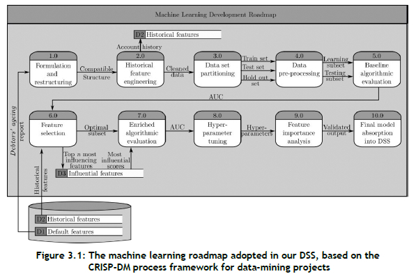
The machine-learning methodology embedded in our DSS was broadly inspired by the well-known cross-industry standard process for data mining (CRISP-DM) framework proposed by Wirth and Jochen [17], which has since become the de facto industry standard for carrying out data-mining projects. The framework served as the basis for our design of a roadmap to guide analysts in developing an effective and efficient tool for solving instances of the IPPP. The roadmap is illustrated graphically in Figure 3.1.

Step 1.0 in the roadmap involves formulating an instance of the IPPP by gaining an understanding of the business question underlying the problem instance in terms of an appropriate data set. This also includes restructuring the data set so that it is possible to address the aforementioned business question by the application of suitable machine-learning models. Step 2.0 involves engineering historical features in order to leverage previous regular customer behaviour during the subsequent analysis. Thereafter, the data set is partitioned into suitable training, test, and hold-out sets in Step 3.0. This is followed in Step 4.0 by applying necessary data pre-processing techniques in order to address potential data quality problems. Step 5.0 of the roadmap, baseline algorithmic evaluation, involves training and testing a selection of machine-learning candidate models on all features contained in the initial data set (which excludes the engineered features). The returned algorithmic performances are taken as a baseline against which candidate models may later be compared. The next step, Step 6.0, involves subjecting the entire data set to a feature selection process with the objective of arriving at an optimal subset of predictive features in Step 7.0. The following step (Step 8.0) is devoted to tuning the hyper-parameters of a suite of candidate machine-learning models under consideration with a view to optimising their prediction accuracy. The aforementioned phases of pre-processing and analysis are often performed iteratively during any data-mining project, and the context of the IPPP is no exception. That is, if the candidate models' performances are not deemed satisfactory, the analyst has to revert to appropriate previous steps. The penultimate step of the roadmap, Step 9.0, involves conducting a feature importance analysis in which the objective is to ascertain the weights that predictive features carry with respect to the outcome of the target feature (i.e., the time period during which invoice payment is expected). The machine-learning roadmap concludes in Step 10.0 with an absorption of a final machine-learning model into the DSS by selecting the best performing model from the set of candidate models.

3.2. DSS derived from the machine-learning development roadmap

The roadmap of the previous section allows for the consideration of a variety of machine-learning models by which to carry out the learning process described above. Such implementations, however, are typically of value and accessible only to those who possess sufficient technical skills related to accounts receivable and/or machine-learning modelling. This section is therefore devoted to a detailed description of a (theoretical) DSS based on the roadmap of the previous section, which is aimed at rendering the predictive power of machine learning that is available to relevant stakeholders of the IPPP.

3.2.1. Proposed functionalities of the decision support system

A process model of our proposed DSS architecture is elucidated in the form of a data flow diagram in Figure 3.2. The figure contains a graphical representation of the inputs, processes, and outputs of the system, based on the development roadmap described in §3.1.

 

 

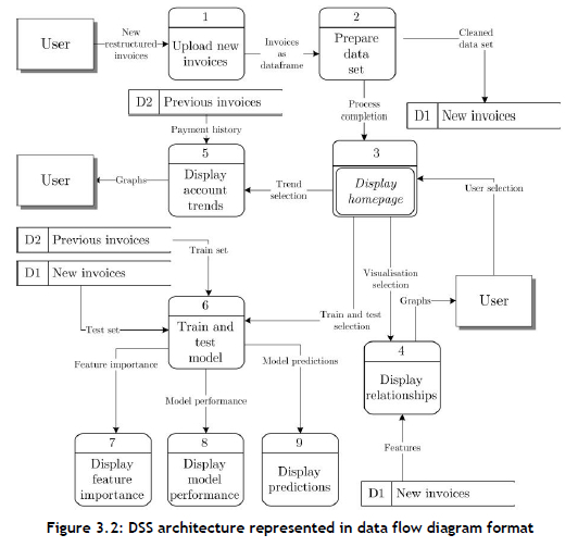
The DSS adheres to four desirable functional requirements: (1) It is able to auto-clean a given data set; (2) it is capable of visualising relationships between selected variables in the data set; (3) it has the ability to predict the outcome of newly created invoices; and (4) it is able to display these predictions. The remainder of the discussion in this section is devoted to an elaboration of the various functionalities that we propose for inclusion in the DSS with the objective of meeting its functional requirements.

Upon launching the system, we recommend that five communication tabs be made available to the user to navigate between the pages of the DSS in order to facilitate simple navigation. The first tab should prompt the user to upload data on new invoices issued. Once loaded, the system should automatically construct historical features pertaining to the data set. Thereafter, pre-processing of the data set should follow. The user should be notified when the two processes are complete. Functionality should also be provided to allow the user to initiate the processes of training and testing machine-learning models.

A second tab should enable the user to visualise the relationships between the aforementioned features in two separate plot areas. The first should contain a scatter-plot matrix of two or more data features selected by the user in which each point is represented on a Cartesian plane, with its colour representing one of the target variable classes. The purpose of such a plot area is to enable the user to obtain a high-level overview of the inherent relationships that are present in the data set. The second plot area should allow the user to visualise any two selected features against each other in a similar manner, but with the added functionality of being able to plot the distributions of each individual variable by invoking various types of visualisations. These visualisation options might include boxplots, histograms, rug plots, and violin plots.

The third tab should contain similar plot areas, but this time to illustrate the payment history of customers, which is also employed as the training set of the machine-learning models. The first plot area should contain a line plot of the average number of days invoices were paid late out of all the customers, from the earliest date in the data set to the current date. The second plot should depict the number of days a payment was paid late for a specific account selected by the user.

We propose that the fourth tab consist of two main components: a stacked bar chart and a table. The bar chart should summarise the predictions made by any particular machine-learning model per target variable category. More detail could be provided per prediction for the invoices in the table, such as general information per account, the predicted target class (i.e., the anticipated period of payment receipt), and the probabilities of the invoice belonging to each of the target classes. The user should also be afforded the ability to alter and sort the predicted outputs, which might help to prioritise debt collection resources. Finally, the user should be afforded the ability to download the full table in case further analysis is necessary on another platform.

The fifth and final tab should contain a bar graph depicting the feature importance measures returned by the machine-learning models. Moreover, a web-application should ideally be chosen as the platform for development so that multiple users are able to access the DSS service remotely.

3.2.2. Proposed verification of any instantiation of the DSS

The objective of verifying a computerised DSS instantiation is to test whether the system has been implemented correctly. The system development should be documented by means of commented sections within the implementation code in case future programmers should be interested in improving upon or extending the functionality of the DSS instantiation. This also facilitates the process of removing syntax errors and compiling errors throughout system development.

Because logical errors are not easily identified, we propose that a structured approach to testing for such errors be followed, such as the approach suggested by Kendall and Kendall [18]. This approach has four steps. The first, program testing with test data, involves developing each component of the DSS instantiation independently and evaluating its functionalities in the context of synthetic data. Moreover, the outputs of each individual component of the instantiation should be compared in isolation with the output provided during each step of the machine-learning development roadmap of §3.1, ensuring that the outputs correspond (this should include the feature-engineering process, the data-cleaning process, and the model-training process). The synthetic data used during this step should also serve the purpose of testing the implemented system's response to violations of the minimum and maximum allowable values that the data can assume.

The second verification step of Kendall and Kendall [18], link testing with test data, should be applied next to verify all communication between the various phases and processes depicted in the data flow diagram of Figure 3.2. This could be achieved by evaluating whether each input provided by the user correctly translates into a change in downstream processes. This includes, for example, uploading hypothetical invoice instances and evaluating whether they result in the correct test set for a machine-learning algorithm after first having been subjected to the feature-engineering and data-cleaning processes.

The working of the entire DSS instantiation should then be subjected to careful testing during the third verification step, full systems testing with test data. The main objective of this step is to evaluate whether the outputs have been visualised correctly via the user interface of the implemented system.

Last, full systems testing with live data should be conducted in tandem with system validation on a holdout set. The hold-out set presents the DSS instantiation with real data so as to assess whether its outputs accurately represent the parameters of the underlying real-world system.

 

4. DEMONSTRATIVE CASE STUDY

In this section, the actual use and applicability of a particular computer implementation of the DSS proposed in the previous section are demonstrated in the form of a case study based on real-world invoice data provided by Curro Holdings Ltd (hereafter referred to merely as 'Curro'), a provider of primary and secondary schooling in South Africa. The case study opens in §4.1 with a brief background discussion of Curro and the context of the data set it provided. A deeper analysis of the data is then conducted in §4.2, based on steps 1-4 of the development roadmap proposed in §3.1. Steps 5-10 of the roadmap are followed thereafter in §4.3 during a discussion of the processes that were adopted to evaluate a variety of machine-learning candidate models with a view to building an appropriate machine-learning model that was tailored to the particular IPPP instances experienced at Curro. The final section of the case study, §4.4, is devoted to an evaluation and validation of the model-driven DSS, based on a hold-out data subset.

4.1. Background to the case study

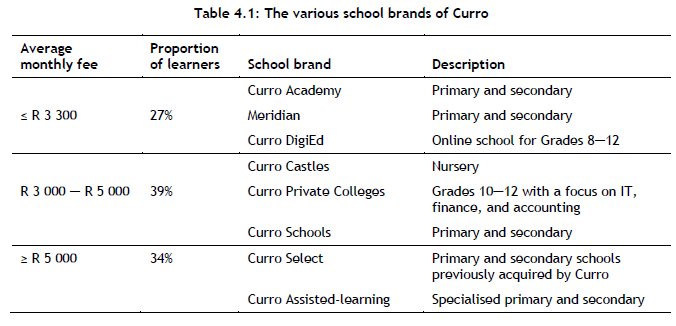
Curro, the industry partner on which this case study is based, was established in 1998 as a for-profit organisation that designs, constructs, and manages independent schools for children from the age of three months to Grade 12. The company's vision is "... to make independent school education accessible to more learners throughout Southern Africa" [19]. Since its inception, the company has enjoyed impressive growth - from having only five campuses and around 3 000 learners in 2010 to boasting 62 698 learners in 2019, spread across 76 campuses (175 schools) [19]. Curro offers numerous school brands to a variety of customers, as summarised in Table 4.1.

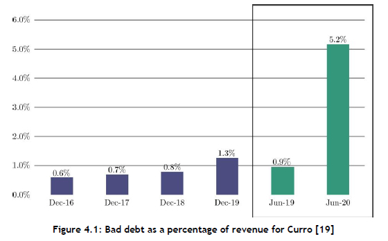
Curro's growth has, however, not been without challenges. As a for-profit organisation, Curro's financial success depends on the size of its client base, which consists of parents paying school fees. Unfortunately, the recent economic downturn in South Africa has seen an increase in the rate of unemployment, from 24.69% in 2010 to 28.48% in 2020. Moreover, the impact of the Covid-19 pandemic has placed strain on South African families on multiple fronts - not just financially. Multiple lockdowns during 2020 forced children to stay at home and attempt to learn remotely, which was a significant challenge, especially for children in low- to medium-income households who might not enjoy an ideal learning environment at home. The challenges of 2020 have forced parents to make tough decisions about whether or not to discontinue their children's education. All these phenomena have culminated in a situation in which many parents have been either unable or unwilling to pay their children's school fees on time. If a customer of Curro (i.e., a parent) fails to pay off debt over an extended period, the debt is written off as bad debt. Curro's bad debt as a percentage of revenue has increased significantly of late, as may be seen in Figure 4.1.

 

 

The data set provided to the authors by Curro contains entries from two of its eight brands - namely, the Curro Schools brand1 and the Curro Academy brand. These brands function independently, differ in both their target markets and monthly school fees, and are therefore considered likely also to exhibit different customer payment behaviours. For this reason, machine-learning analyses were conducted separately for each school brand.

The data set contained 1 068 620 invoice entries from the period from January 2016 to April 2021. It comprised twenty descriptive features and a single multi-class target feature exhibiting a payment-on-time category (0 days late) and three late-payment categories, distributed as shown in Figure 4.2. The descriptive features constituted ten categorical features and ten continuous features. These features represent financial and limited demographic information in respect of each account holder. The names and brief descriptions of all of the features in the training set are tabulated in Appendix A at the end of this article.

An important distinction has to be made between invoices generally issued by companies and invoices issued by Curro. In the more general case, invoices differ in the amounts owed by customers, while in the case of Curro, a standardised invoice is issued to all customers at a given school. This means that families with varying financial capabilities are required to pay the same amount towards school fees.

Owing to the large volume of data available to Curro on a customer level, a machine-learning model may profitably be used to predict individual customer invoice payment behaviour. By identifying invoices likely to become delinquent at the time of issue, this knowledge could be used to adopt a focused approach to the collection of debt. If, for example, a high probability of delinquency is predicted for a particular invoice, the time to collection can be reduced by pro-actively attempting to collect on that invoice. Such an ability is anticipated to be especially valuable in situations where resources for collection activities are limited. Ultimately, a predictive model might well lead to an increase in Curro's financial stability and to improved customer payment behaviour - an outcome that would be advantageous to Curro, its parents, and its learners.

1 Also colloquially referred to merely as 'Curro'. While this brand name should not be confused with the name of the entire company, it will be clear from the context when the word Curro refers to the brand or to the entire company.

4.2. Customised DSS instantiation

A computerised instantiation of the DSS proposed in Section 3 was developed for Curro in Python, along with a graphical user interface designed according to the functionality guidelines of §3.2.1. Python was chosen for this purpose because it is now regarded as the de facto language for machine-learning applications [20], surpassing other languages such as R and Java [21]. Moreover, the software environment's thriving online community provides a wealth of knowledge that can be consulted and referenced during any data-mining project. The specific software environment selected was Dash, a user interface library for creating web applications that is commonly used during data science projects [22]. Our DSS instantiation allows users to interact with graphs by providing functionalities such as the ability to download figures, display data points when the cursor hovers over a graph, and update outputs based on user-specified inputs. We used this instantiation to perform the data set analysis and machine-learning model evaluation.

4.3. Data set analysis

In order to obtain a suitable machine-learning model capable of predicting customer behaviour in the DSS, the Curro data set first had to be analysed, understood, and transformed into an appropriate format. The subsections contained in this section correspond with steps 1-4 of the machine-learning development roadmap proposed in §3.1.

4.3.1. Formulation and restructuring

The formulation and restructuring step of the roadmap entailed converting the structure of the input data set from a report into one that was suitable for machine-learning analyses. Thereafter, the data could be explored and the learning problem formulated.

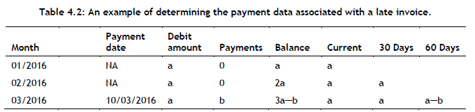
Upon conducting an initial investigation into the data provided by Curro, numerous anomalies were detected that rendered the structure of the data incompatible with the application of a machine-learning algorithm aimed at predicting when future invoices would be paid. The main cause of these anomalies was that the data were provided in a format commonly known as an accounts receivable report [23]. Such a report format is adopted by companies to ascertain the financial health of their customers by categorising customer invoices based on the length of time they are outstanding. The format typically involves columns representing intervals of 30 days, and shows the amount payable over these intervals [21]. For example, if an invoice is not paid within 30 days, the amount owed is moved to the column corresponding to the next interval, resulting in an increase in the total amount payable, as illustrated in Table 4.2.

Consequently, the next entry, or invoice, contains information about the outcome of the previous entry - a property that violates the requirement of machine-learning algorithms that all observations should be independent of one another. Thus a number of changes were made to the overall structure of the data.

The first irregularity detedted was that the payment dates of the invoices issued were not contained in the associated columns of that row. A search algorithm therefore had to be designed to determine the payment date of each invoice. In the event of a payment, the amount paid was subtracted from the oldest outstanding invoice, as illustrated in the third entry of Table 4.2. The algorithm was required to exhibit different behaviours in three fundamentally distinct cases (as described in more detail in Appendix B):

• (Case I) An invoice is paid late,

• (Case II) An invoice is paid in advance, and

• (Case III) An invoice is paid during the required month

Another anomaly detected was that multiple transactions were often issued in respect of the same account for a given month. This was mainly because parents had accounts for more than one learner or received credit for an offered discount. These transactions were combined for each month in a given account so as to result in a combined net invoice.

Once the data had been restructured as described above, and the payment dates for each respective invoice had been calculated, the number of days a payment was late could be calculated by subtracting the invoice date from the payment date. This was achieved by binning these variables into bins that aligned with the intervals of the accounts receivable report, leading to the type of analysis that then had to be performed being classified as a multi-class classification problem. An analysis was carried out to ascertain the distribution of the payments for each interval, as shown in Figure 4.2. An interval value of 0 days indicated that the invoice was paid in advance (Case II), and accounted for 45.19% of the total number of invoices issued. Training a prediction algorithm on these data entries was trivial, since a simple subtraction would suffice when the invoice was issued to determine whether it had been paid in advance. As a result, all of these entries were removed from the data set.

4.3.2. Historical feature engineering

As explained in Section 2, similar studies in the literature have shown that the introduction of features capturing historical behaviour resulted in an increase in prediction accuracy of between 9% and 27%. Such an application might prove to be especially useful in the Curro training set, considering that, on average, there were 29 invoices per account in the data set, resulting in an abundance of historical information. The obvious constraint is that such an application is not viable for the first invoice of an account, since there is no historical information available for that invoice. These features were, therefore, only created for invoices for which previous information was available. The first entry of each account was subsequently removed from the analysis. Table 4.3 contains information about the features that were generated. These features were loosely based on features considered in the studies described in Section 2.

Features 1 -4 were generated with the objective of capturing general outcomes related to previous invoices. Moreover, features 5 and 6 were generated to represent the timings of payments made by the account holder. The purpose of features 7 and 8 was to capture recent customer behaviour. Last, the purpose of feature 9 was to capture global trends in invoice payments during previous months.

The calculation of features varied according to how many invoices were included and the weighting of each invoice. When calculating AveDaysLate, for example, the value was simply calculated as the mean value over all previous invoices. Such a calculation is, however, unresponsive to recent changes in payment behaviour. If too much weight is allocated to recent behaviour, on the other hand, then the value might respond to noise.

A suitable method of calculating historical values was determined empirically by evaluating the classification accuracy achieved by a simple random forest model in respect of three different calculation methods. First, the mean over all previous invoices was calculated. Second, the mean over a fixed number of previous invoices was calculated. This specified length, or window size, ranged from two to five. Last, the features were calculated as the weighted average of the previous ten invoices. The weights were assigned according to factors specified a priori. For example, if the value were to be 1.2, then each value would contribute 1.2 times as much to the metric as the next invoice further away from the calculation instant.

Of these permutations, the exponential weighting method yielded the best prediction accuracy. Weight factors in the range [1,2] were considered and tested empirically in discrete steps for their ability to promote prediction accuracy. A factor value of 1.5 was found to perform best.

4.3.3. Data set partitioning

There are various ways in which data sets have traditionally been partitioned by means of sampling [2]. Traditional techniques could not, however, be implemented in the context of the Curro data set, since the time-series nature of the data set created the risk of a data leakage.

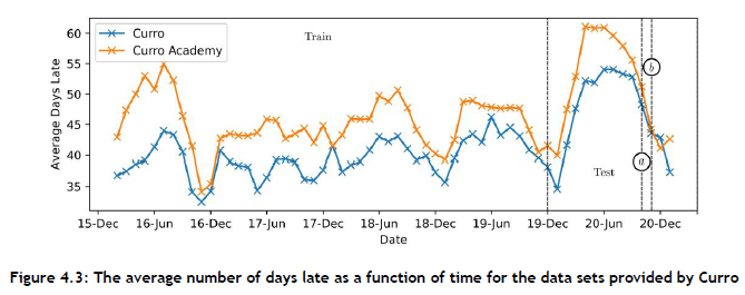
Therefore, the data set was partitioned according to time. The selected training set corresponded to invoices from 2016 to 2019, representing 56% of the data set, while the selected test set corresponded to all invoices for 2020, or 32% of the data set. The set used for the tuning of hyper-parameters was all invoices issued during October 2020, represented by the slice denoted a in Figure 4.3, which elucidates the average number of days late of all accounts over time. A separate hold-out set corresponded with invoices issued during November 2020, represented by the slice b in Figure 4.3. The purpose of this hold-out set was to facilitate unbiased testing and verification of the DSS instantiation. Invoices issued in 2021 did not form part of the analysis, since the corresponding payment outcomes did not reflect yet in the data set.

The process of testing a variety of machine-learning models resembled a simulation of the actual functioning of the DSS. The models were required to make predictions for all newly created invoices at the beginning of a month, and were trained on all invoices prior to that. In order to obtain an accurate measure of the models' performances, predictions were made for each month of the calendar year 2020. That is, the models were trained on the 2016 to 2019 data, and were required to make predictions for January 2020. Thereafter, the models were re-trained on all data spanning the period from 2016 to January 2020, and were required to make predictions for February 2020, and so forth. The mean performance over all twelve prediction months was then taken as the performance measure associated with a model.

The seasonal nature of the data justified predicting only one month into the future, as illustrated in Figure 4.3. If retrained on a monthly basis, the model is expected to be able to develop the capability of responding to changes in customer behaviour - especially in the presence of a significant external shock, such as the disruption caused by the Covid-19 pandemic in 2020. Such frequent retaining is natural (in the sense that it coincides with the frequency of issuing invoices) and should not impact the user of the DSS instantiation negatively, because training can easily take place overnight at the end of each month so that the system is ready for updated use once new invoices are issued (retraining of only a single machine-learning algorithm is required).

4.3.4. Data pre-processing

A data quality report formed the basis for addressing data quality issues early on in the data-mining process [2]. The report tables were scrutinised to gain a deeper insight into the nature of the data and subsequently to identify quality concerns.

Each feature was inspected with a view to identifying errors. The first problem to be identified was that the payment date searching algorithm could not find the payment dates for 9% of the entries. This anomaly was found to represent errors, since the rules of the accounts receivable report had been violated. The relevant entries were subsequently removed.

A second issue related to the distribution of the Age feature, the OldestLearnerAge and FirstLearnerStart features, and the ActualAmt feature. These errors were eliminated either by the method of mean imputation or by removing all instances containing values larger than or smaller than sensible threshold values.

It also became apparent from the data quality report that two features were associated with large proportions of missing values, and these features were subsequently removed. The features were ParentalRelationship and IncomeBracket, exhibiting missing value percentages of 57.5% and 99.5% respectively.

Upon inspection of the minima, maxima, and standard deviations of the continuous features in the data quality report, it also became evident that outliers were present in the data set. All outliers were addressed by performing clamp transformation.

From Figure 4.2 it may be concluded that the data sets exhibited class imbalance. Various sampling methods were employed to address this imbalance in an effort to identify the best sampling method: random under-sampling, random oversampling, SMOTE, and Tomek links [24, 25]. A focus was placed on under-sampling techniques, since the number of data entries allowed for such an application. The best method was determined empirically by identifying which method resulted in the best performance for a simple random forest algorithm. The best method of sampling was identified as Tomek links with a resulting class distribution of 50%, 26%, 24% for the Curro brand, and 43%, 29%, 28% for the Curro Academy brand.

Several features were also included in the data set that exhibited irregular cardinalities. For example, a cardinality of 1 associated with the SchoolCountry feature rendered it redundant, and so the feature was removed. The Occupation feature similarly exhibited an extreme cardinality value of 6 378. Because there is not a method for transforming this feature to a sensible continuous feature, it was removed from the data sets. Moreover, the cardinality value of 10 for the ParentalRelationship feature raised concerns over the discriminating information it provided. A total of 57.5% of the entries were missing, which further diminished the useful information it represented. The feature was therefore also removed.

Several other pre-processing methods were also applied to the data sets. First, all categorical variables that were not ordinal, and that contained two or more categories, were continuised by applying the method of one-hot encoding [26]. The only feature that met the requirements for this type of transformation was the SchoolRegion feature. The data were further normalised for the models that required this type of transformation. Two normalisation techniques, standardisation and robust scaling, were applied [25, 27]. The best normalisation technique was determined empirically for each of the machine-learning models.

4.4. Machine-learning model evaluation

Once the data had been pre-processed, the training and evaluation of a suite of machine-learning candidate models could take place. The subsections contained in this section correspond with steps 5-10 in the development roadmap of §3.1.

4.4.1. Baseline algorithmic evaluation

A total of six classifiers were first trained on the standard data sets (excluding the engineered features) in order to establish baseline algorithmic performances. These classifiers were a random forest model, a decision tree model, the k-nearest neighbour algorithm, logistic regression, a naive Bayes classifier, and a dense neural network. The performance measure that was considered when evaluating each of these algorithms was the well-known area under the receiver operating characteristic curve, abbreviated here as AUC. This measure forms part of the widely popular machine learning library for data-mining projects written in Python, called scikit learn. This measure exhibits flexibility in respect of accommodating multi-class classification, and provides robust performance measures in the case of class imbalance. For the purposes of this case study, the average (unweighted) AUC was computed for all possible pairwise combinations of classes, as recommended by Pedregosa et al. [28].

4.4.2. Feature selection

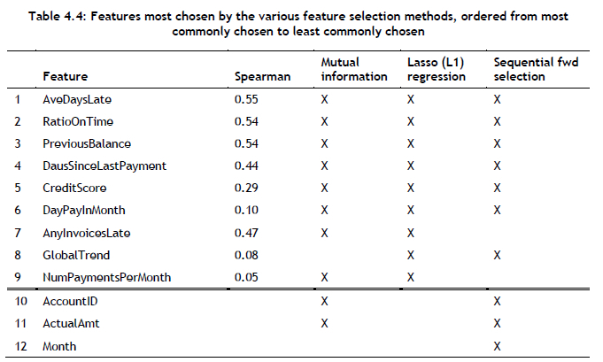
The data sets were subsequently enriched with the historical features that had been engineered. Thereafter, feature selection was performed on all of the data sets in an attempt to arrive at an appropriate number of features. For feature selection, two filter methods, one wrapper method, and one embedded method were used during training. The two filter methods were Spearman correlation [5] and mutual information [29]. The wrapper method employed was sequential forward selection, with a random forest model [30] adopted for evaluation purposes. Finally, the embedded method employed was Lasso (L1) regression [26]. The results are tabulated in Table 4.4, with the features sorted from most commonly chosen to least commonly chosen. Features were included for further analysis if they were present in the results returned by at least three out of the four selection methods. Features 1-9 in Table 4.5 were, therefore, selected.

 

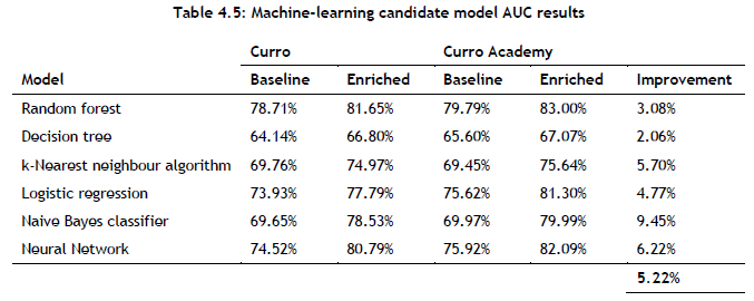
4.4.3. Enriched algorithmic evaluation

The respective models were re-trained and tested with respect to the selected subset of features determined during feature selection. Table 4.5 contains a comparison between the AUC scores achieved by the baseline models and the AUC scores achieved by the enriched models. From the table it is evident that the feature selection and feature engineering processes resulted in an increase in prediction accuracy for all models - most notably for the naive Bayes classifier, the k-nearest neighbour algorithm, and the dense neural network.

4.4.4. Hyper-parameter tuning

Most machine-learning models contain parameters that have to be specified a priori and that influence model prediction accuracy. This type of model parameter is called a hyper-parameter, and is typically tuned empirically, since there is no analytic method for calculating appropriate values for hyperparameters [31]. The hyper-parameter tuning process followed for the different machine-learning models involved use of the widely adopted method of grid search. This method entails considering all distinct hyperparameter value combinations in a pre-defined and discrete search space. Ranges for the various hyper-parameters were derived from guidelines in the literature, upon which small, medium, and large values were selected for consideration within these ranges. The method can become prohibitively expensive, however, if there are many hyper-parameters. For this reason, the test set employed during hyper-parameter tuning only contained one month of invoice data, instead of aggregating the performances for the entire 2020 calendar year. It is acknowledged that other hyper-parameter tuning approaches could have been implemented instead, such as Latin hypercube sampling, a sensitivity analysis, or Bayesian evidence-based tuning. The hyper-parameters relevant to each algorithm, as well as the best performing combination of hyper-parameters for each Curro brand, may be found in Appendix C.

4.4.5. Feature importance

A variable importance analysis was performed in respect of the best-performing machine-learning models identified in the previous section. The objective was to identify features that were deemed to be most predictive of invoice payment behaviour. In the previous section, the random forest model was identified as exhibiting the best performance in prediction accuracy, and so this model is mainly evaluated in this section. For the sake of brevity, only the tuned random forest model employed for the Curro Academy brand is considered (the models for the two brands differed only marginally).

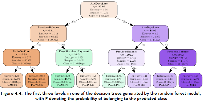
The structure of the first three levels of one of the trees produced by the random forest model is illustrated graphically in Figure 4.4.

The first feature adopted by the random forest model to perform splitting was the AveDaysLate feature. A value for this feature of more than 49.05 was found to increase the probability of an invoice being paid late. It is interesting to note that, if the value of the AveDaysLate feature is larger than 84.03, and the value of the PreviousBalance feature is larger than 3 001.5, the invoice has a probability of 89.3% of being at least 61 days late. This indicates that customers who have a history of paying invoices late and have outstanding invoices (larger positive balances) are very likely to pay these invoices more than two months after their issue date. Conversely, customers who have a history of paying on time, and have a healthy balance, are likely to pay earlier.

In order to calculate the feature importances for the (multinomial) logistic regression model, the absolute coefficients associated with the respective features were normalised. The other three algorithms are not inherently capable of providing feature importances. To overcome this limitation, the notion of permutation importance was employed. Permutation importance involves randomly shuffling a single feature in the data set while leaving the rest of the data set intact, and comparing a model's prediction accuracy with the baseline [32]. If variables that contain predictive information are shuffled, it will lead to poorer performance and a higher feature importance value. The normalised results obtained are represented in Figure 4.5.

It is evident that the first three features - AveDaysLate, RatioOnTime, and PreviousBalance - were deemed to be important variables in predicting the outcome of invoice payments by all of the models apart from the logistic regression model, which returned a large coefficient for the AnyInvoicesLate feature, possibly owing to the linear relationships it assumed between variables, unlike the other models.

The features that contributed only marginally towards predictability, on the other hand, were the DaysSinceLastPayment, NumPaymentsPerMonth, DayPayInMonth, and GlobalTrend features. In other words, when customers last made payments, how often they make payments, when their payments occur during the month, and the global trend of payments during the previous month only have a marginal effect on the invoice payment outcomes.

4.4.6. Final absorption of model into the DSS

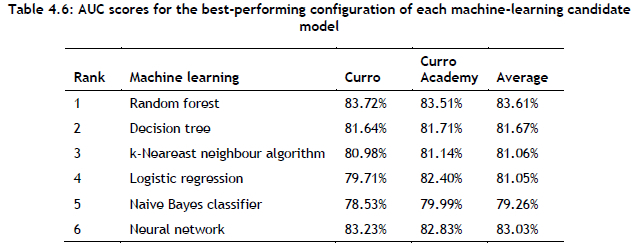
The AUC scores of the best-performing configurations of each machine-learning candidate model are summarised in Table 4.6. Although the relative differences between the AUC scores decreased between the respective models, the best-performing algorithm for both brands was again determined to be the random forest model. This model was therefore considered for absorption into the DSS instantiation. The option of ensembling machine-learning models was not pursued, since it would be associated with a considerable increase in computational burden.

4.5. Embedding the random forest model into the DSS

Having absorbed the random forest model into the DSS instantiation, the applicability and performance of the instantiation as a whole could be evaluated. A brief analysis of how the system performed on the holdout set is first elaborated upon. This is followed by a description of the feedback received during an expert face validation of the DSS results pertaining to the hold-out set.

4.5.1. Experimental results on hold-out set

The hold-out set was employed during a final evaluation of the model-driven DSS instantiation. It also formed the basis for obtaining an expert face validation from subject matter experts (SMEs). The AUC scores returned by the random forest models were 79.01% for the Curro brand, and 82.5% for the Curro Academy brand.

4.5.2. Expert face validation

The purpose of system validation is to ensure that an appropriate system has been built that exhibits the required level of sophistication and fidelity [33]. Most importantly, it entails evaluating whether the system accurately models the underlying real-world system. An important step in system validation, apart from experimental validation, is ensuring that the system achieves high face validity. This typically entails the involvement of an SME who is consulted to determine whether the system imitates the underlying physical system accurately.

The main SME selected to perform the expert validation was Mr Craig Nel [34], a debt collection consultant with more than twenty years of experience in the industry. He was selected as the main SME for this study because of his considerable knowledge of the fundamental business question underlying the IPPP. An additional SME who also provided valuable input was Ms Monica Rolo [35]. She obtained a master's degree in industrial engineering at Stellenbosch University in 2019 with a thesis topic on unsupervised machine learning. In her role as an industrial engineer at Curro, she has worked on numerous data science projects.

Nel was surprised to note the application of data-driven solutions to debt collection - something he believed to be novel. He noted that the feature importance values returned by the model aligned with the anecdotal evidence that was observed. He also confirmed that the probabilities of an invoice belonging to each target variable class returned by the DSS instantiation would aid in prioritising intervention strategies for invoices that were at the highest risk of defaulting. From a machine-learning perspective, Rolo endorsed the steps followed in the machine-learning development roadmap, as well as the six candidate machine-learning algorithms that were considered. Both SMEs submitted that the distribution of the predicted target feature classes, together with their associated probabilities, were representative of a typical batch of invoices issued during any month.

In summary, the SMEs endorsed the underlying assumptions of the DSS instantiation and confirmed that the results that were returned accurately represented the underlying real-world system.

 

5. CONCLUSION

In this paper, a DSS was proposed for predicting customer payment behaviour in respect of invoices issued. The DSS takes as its input data pertaining to invoices issued for each account of an organisation at the beginning of each month, and provides as output the predicted intervals of payment along with the respective probabilities of payments occurring in each interval. The DSS then proceeds to engineer features that capture the historical behaviour, based on outcomes in relation to previous invoices, saved as a data store. The DSS also facilitates the application of the necessary pre-processing steps in order to train and test the machine-learning model embedded within it. In addition, the DSS is able to provide visualisations of the features contained in the data set, along with the historical trends of payments, with the objective of extracting meaningful relationships between them. The DSS provides output in a meaningful way by enabling users to sort and filter predictions so that debt collection intervention strategies can be prioritised for invoices exhibiting the highest risk of being paid late. Last, the DSS facilitates visualisation of the feature importance values returned during the predictions made by the underlying machine-learning model.

Moreover, a customised instantiation of the DSS was implemented for Curro on a personal computer, and verified. It was demonstrated that the DSS instantiation is able to provide results in the context of a real-world case study, based on data provided by Curro. The model returned AUC scores of 79.01% for the Curro brand and 82.5% for the Curro Academy brand during a case study. The instantiation was judged to hold the potential of resulting in a decrease in bad debt for Curro - a recent and serious phenomenon. The notion of applying data-driven decision support to predict customer payment behaviour is a novel solution, as confirmed by the limited literature related to similar applications and by the anecdotal evidence provided by two SMEs.

As in any predictive system, predicting invoice payment behaviour requires knowledge of previous accounts, and is therefore geared towards predicting the behaviour of existing customers with known data instead of predicting the payment behaviour of new customers. Although the DSS is based on several simplified assumptions, a computerised instantiation of the system was still able to predict invoice payment behaviour with between 79.01% and 82.5% accuracy.

 

REFERENCES

[1] Salek, J.G. 2005. Accounts receivable management best practices, Hoboken, NJ: John Wiley & Sons.         [ Links ]

[2] Kelleher, J.D., Namee, B.M. & D'Arcy, A. 2015. Fundamentals of machine learning for predictive data analytics, 1st ed. Cambridge, MA: MIT Press.         [ Links ]

[3] Piatetsky-Shapiro, G. 2007. Data mining and knowledge discovery 1996 to 2005: Overcoming the hype and moving from university to business and analytics. Data Mining and Knowledge Discovery, 15(1), pp 99-105.         [ Links ]

[4] Khandani, A., Kim, A. & Lo, A. 2010. Consumer credit-risk models via machine-learning algorithms. Journal of Banking and Finance, 34, pp 2767-2787.         [ Links ]

[5] James, G., Witten, D., Hastie, T. & Tibshirani, R. 2013. An introduction to statistical learning. New York, NY: Springer.         [ Links ]

[6] Gambacorta, L., Huang, Y., Qiu, H. & Wang, J. 2019 How do machine learning and non-traditional data affect credit scoring? New evidence from a Chinese fintech firm. Bank for International Settlements Working Paper, 834, pp 1-20.         [ Links ]

[7] Zeng, S., Melville, P., Lang, C., Boier-Martin, I. & Murphy, C. 2008. Using predictive analysis to improve invoice-to-cash collection. In Proceedings of the 14th ACM SIGKDD International Conference on Knowledge Discovery and Data Mining, Las Vegas, NV, pp 24-27.         [ Links ]

[8] Lee, E.T. & Wang, J. 2003. Statistical methods for survival data analysis. Hoboken, NJ: John Wiley & Sons.         [ Links ]

[9] Smirnov, J. 2016. Modelling late invoice payment times using survival analysis and random forests techniques. PhD thesis, University of Tartu, Tartu.         [ Links ]

[10] Nisbet, R., Elder, J. & Miner, G. 2009. Handbook of statistical analysis and data mining applications. San Diego, CA: Elsevier.         [ Links ]

[11] Appel, A.P., Oliveira, V., Lima, B., Malfatti, G.L., De Santana, V.F. & De Paula, R. 2019. Optimize cash collection: Using machine learning to predicting invoice payment. [Online] Available from https://arxiv:org/pdf/1912:10828:pdf. [Accessed 17 April 2021].         [ Links ]

[12] Bramer, M. 2007. Principles of data mining. New York, NY: Springer.         [ Links ]

[13] Perko, I. 2017. Behaviour-based short-term invoice probability of default evaluation. European Journal of Operational Research, 257(3), pp 1045-1054.         [ Links ]

[14] Nielsen, M.A. 2015. Neural networks and deep learning. San Francisco, CA: Determination Press.         [ Links ]

[15] Engelbrecht, A.P. 2007. Computational intelligence: An introduction. Pretoria: John Wiley & Sons.         [ Links ]

[16] Hosmer, D.W. Jr & Lemeshow, S. 2000. Applied logistic regression. New York, NY: Wiley.         [ Links ]

[17] Wirth, R. & Jochen, H. 2000. CRISP-DM: Towards a standard process model for data mining. In Proceedings of the 4th International Conference on the Practical Applications of Knowledge Discovery and Data Mining, Manchester, pp 29-39.         [ Links ]

[18] Kendall, K.E. & Kendall, J.E. 2011. Systems analysis and design, 9th ed. Upper Saddle River, NJ: Pearson Prentice Hall.         [ Links ]

[19] Curro Holdings Ltd. 2019. Curro, Annual integrated report. [Online] Available from m https://www:curro:co:za/media/206947/curro-holdings-ltd-annual-integrated-report-ye2019:pdf. [Accessed 27 March 2021].         [ Links ]

[20] Srinath, K. 2017. Python - The fastest growing programming language. International Research Journal of Engineering and Technology, 4(12), pp 354-357.         [ Links ]

[21] Louw, M. 2021. Financial manager at Curro Holdings Ltd. [Personal communication]. Contactable at marietjie.l@curro.co.za.         [ Links ]

[22] Globe News Wire. 2019. Plotly announces newest version of Dash Enterprise Analytic Application Deployment Platform. [Online], Available from https://www:globenewswire:com/news-release/2021/10/14:html. [Accessed 7 July 2021].         [ Links ]

[23] Hellerstein, J. 2021. Quantitative data cleaning for large databases. [Online]. Available from https://citeseerx:ist:psu:edu/viewdoc/download?doi=10:1:1:115:6419&rep=rep1&type=pdf. [Accessed 12 June 2021].         [ Links ]

[24] Batista, G.E., Prati, R.C. & Monard, M.C. 2004. A study of the behavior of several methods for balancing machine learning training data. ACM Explorations Newsletter, 6(1), pp 20-29.         [ Links ]

[25] Haibo, H. & Yunqian, M. 2013. Imbalanced learning: Foundations, algorithms, and applications. Piscataway, NJ: IEEE Press.         [ Links ]

[26] Kuhn, M. & Johnson, K. 2019. Feature engineering and selection: A practical approach for predictive models. London: Taylor & Francis.         [ Links ]

[27] Bellman, R. 1969. A new type of approximation leading to reduction of dimensionality in control processes. Journal of Mathematical Analysis and Applications, 27(2), pp 454-459.         [ Links ]

[28] Pedregosa, F., Varoquaux, G., Gramfort, A, Michel, V., Thirion, B., Grisel, O., Blondel, M., Prettenhofer, P., Weiss, R. & Dubourg, V. 2011. Scikit-learn: Machine learning in Python. Journal of Machine Learning Research, 12, pp 2825-2830.         [ Links ]

[29] Chandrashekar, G. & Sahin, F. 2014. A survey on feature selection methods. Computers and Electrical Engineering, 40(1), pp 16-28.         [ Links ]

[30] Pudil, P., Novovicová, J. & Kittler, J. 1994. Floating search methods in feature selection. Pattern Recognition Letters, 15(11), pp 1119-1125.         [ Links ]

[31] Kuhn, M. & Johnson, K. 2013. Applied predictive modeling. New York, NY: Springer.         [ Links ]

[32] Altmann, A., Tolosi, L., Sander, O. & Lengauer, T. 2010. Permutation importance: A corrected feature importance measure. Bioinformatics, 26(10), pp 1340-1347.         [ Links ]

[33] Banks, J., Carson, J., Nelson, B. & Nicol, D. 2010. Discrete event system simulation, 5^th ed. Upper Saddle River, NJ: Pearson.         [ Links ]

[34] Nel, C. 2021. Debt collection consultant at Curro Holdings Ltd. [Personal communication]. Contactable at craig.n@curro.co.za.         [ Links ]

[35] Rolo, M. 2021. Industrial engineer at Curro Holdings Ltd. [Personal communication]. Contactable at monica.r@curro.co.za.         [ Links ]

[36] Hornik, K., Stinchcombe, M. & White, H. 1989. Multilayer feedforward networks are universal approximators. Neural Networks, 2(5), pp 359-366.         [ Links ]

 

 

Submitted by authors 11 May 2022
Accepted for publication 12 Sep 2022
Available online 14 Dec 2022

 

 

* Corresponding author: vuuren@sun.ac.za
ORCID® identifiers
L. Schoonbee: 0000-0002-9386-5753
W.R. Moore: 0000-0002-8032-3584
J.H. van Vuuren: 0000-0003-4757-5832

 

 

APPENDIX A: DESCRIPTIONS OF ALL FEATURES IN THE TRAINING SET

AccountID. The account number of the client

CalenderMonthKey. The date time stamp of the invoice

Brand. The school brand the account is associated with

SchoolCountry. The country in which the school is located

SchoolRegion. The province in which the school is located

ParentalRelationship. Type of relationship between account holder and learner

Occupation. Occupation of account holder

Age. Age of account holder

Gender. Gender of account holder

CreditScore. Credit score of account holder

NumberOfLearnerResponsibleFor. The number of learners for whom the account is responsible

FirstLearnerStart. How long ago the first learner started school

OldestLearnerAge. The age of the oldest learner

ReceivesDiscount. Whether or not an account receives a discount

PaymentMethod. Whether a payment is made via cash or debit order

IncomeBracket. The income bracket of the account holder

InvoiceDate. The date and time stamp of the issue of the invoice

PaymentDate. The date and time stamp of when a payment was received during the month

DebitAmt. The amount debited

CreditAmt. The amount credited

ActualAmt. The net amount

TaxAmt. The tax amount associated with the invoice

Payments. The payment amount

Balance. The balance of the account holder

 

APPENDIX B: CASES CONSIDERED WHEN DETERMINING THE PAYMENT DATE OF EACH INVOICE

(Case I) An invoice is paid late. If the value in the Current column is positive, the algorithm iteratively searches through each row and identifies when an invoice does not appear in the next interval for the following month. In other words, if the payment b is larger than a in the third entry of Table 4.2, this means that the invoice issued in January was paid on 10 March 2016.

(Case II) An invoice is paid in advance. If an invoice was paid during, or before, a given month, the value in the Current column would be non-positive - also implying that all other invoices had been paid. If the balance of the previous month is therefore negative, and the sum of the previous month's balance and the debited amount is still non-positive, then the invoice is considered paid, irrespective of whether a payment occurred during that month. For example, if y + x < 0 in Table B.1, the invoice has been paid in advance and the payment date is set to the invoice date.

 

Table B.1 - Click to enlarge

 

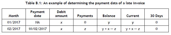
(Case III) An invoice is paid during the required month. If, however, the sum of the previous month's balance and the debited amount is positive, then the invoice was only considered paid when a payment was received during that month, resulting in the Current value being non-positive. To relate this back to the example above, the inequalities y + x > 0 and y + x - z < 0 would hold in this case.

 

APPENDIX C: ALGORITHMIC HYPER-PARAMETER TUNING

During the training of the decision tree model, four hyper-parameters were identified for tuning. The first, maximal tree depth, determines the maximum number of splits that can occur before a leaf node should be formed. A large value typically results in over-fitting the training set, while a small value results in under-fitting. The second hyper-parameter specifies the minimum number of instances in a subset that are required before a split is made on the subset. A large value typically prevents the model from over-fitting. Another hyper-parameter, the minimum number of instances in leaves, prevents a split from occurring at an interior node if the resulting node contains fewer instances than the value of the hyper-parameter. A large value prevents the model from over-fitting. Last, the function that measures the quality of a split can either employ Gini impurity or information gain.

Five hyper-parameters were tuned in the random forest model. The first was the number of trees in the forest. A large number of trees tends to increase prediction accuracy, but also increases the computational time. Second, the maximum number of attributes considered at each split can assume a value of between five and fifty. Third, the minimum number of instances contained in a node before a split is performed can be between two and one thousand. Moreover, the maximum depth of individual trees can assume a number between one and fifty. Last, it can be specified whether sampling should be conducted with or without replacement; the former is known as bootstrapping.

Two hyper-parameters appeared in the logistic regression model - namely, the regularisation type and the regularisation strength. Regularisation is a technique that is employed to prevent over-fitting, and can also be used as a feature selection method. Two widely adopted methods that can be employed are Lasso (L1) and Ridge (L2) regularisation. The strength of the regularisation, denoted by C, can assume any value between 0.001 and 1 000.

The most obvious hyper-parameter that could be altered in the k-nearest neighbour algorithm was the value of k. A large number prevents the model from over-fitting the training set, but too large a value can lead to under-fitting. Another hyper-parameter was the weight function that was used during prediction, which could employ uniform weights or weight points, based on the inverse of the distance between them. Last, the distance metric employed could also be changed, which could be either Euclidean distance or Manhattan distance.

No hyper-parameters had to be tuned for the naive Bayes algorithm. The Gaussian naive Bayes algorithm was determined to be the most suitable implementation.

In order to prevent a neural network from over-fitting - a common phenomenon as the number of epochs progresses - so-called early stopping formed part of the architecture. This mechanism interrupts the training error as soon as the validation error reaches its minimum. What is especially useful about this mechanism is that a patience parameter is introduced that represents the number of epochs over which the model can still be trained with no improvement, after which training is terminated. This was specified to be three epochs, based on a preliminary empirical analysis. The maximum number of epochs was specified as 50, but the early stopping mechanism usually terminated training after five to fifteen epochs. The validation set was taken to be 25% of the training set.

The number of entries on which training is based before the weights are updated, or the batch size, can be adjusted. The number of epochs can also be changed, which is the number of times the entire data set is introduced during training. Moreover, the training optimisation algorithm can also be altered. In addition, the number of neurons in the hidden layer can be varied. Generally speaking, a larger number of hidden neurons causes the network to over-train. The number of hidden layers could also have been altered during the parameter tuning process, but since standard multilayer feed-forward neural networks are, in theory, capable of approximating any function [36], the value of this hyper-parameter was not varied. The neuron activation functions were also tuned before training and testing on a data set. Last, the measure of how fast the weights are updated at the end of each batch, known as the learning rate, was varied. This rate assumes a value between 0 and 1. A larger value typically results in unstable training, while a smaller value holds the risk of the training process only converging towards local optima.

Another hyper-parameter, known as dropout regularisation, involves incurring a penalty in the training objective that is aimed at preventing over-fitting [15]. This was, however, not considered because of the adoption of the early stopping mechanism and the denseness of the neural network architecture.