


Services on Demand
Article
 English (pdf)
 Article in xml format
 Article references
Indicators

Related links
-
 Cited by Google
 -
 Similars in Google
Share

 Permalink
South African Journal of Industrial Engineering
On-line version ISSN 2224-7890
Print version ISSN 1012-277X
S. Afr. J. Ind. Eng. vol.33 n.4 Pretoria Dec. 2022
http://dx.doi.org/10.7166/33-4-2734
GENERAL ARTICLES
Methods for forecasting demand in repairing an airline's repairable line replaceable unit parts
Y. CaoI; Y. LiuII; D. ShenI, *
IDepartment of Transportation Science and Engineering, Civil Aviation University of China, China
IIDepartment of Economic and Management, Civil Aviation University of China, China
ABSTRACT
Scattered failure frequency, variable and complex influencing factors, and a low accuracy in predicting inventory demand are characteristics of line replaceable unit (LRU) parts. Some high-priced repairable LRU (HR-LRU) parts have a considerable impact on the cost of aircraft spare parts.This study presents procedures to identify the optimal model for forecasting the demand for HR-LRU parts. First, a traditional prediction model, seven single measurement models, and four combined models were selected and used to predict failure data. Subsequently, evaluating indexes were selected for assessment to obtain the optimal model. Finally, we compared the actual and predicted values to verify the conclusions drawn during the previous evaluation step. The results indicated that, among the single models, the negative binomial regression model and the Holt-Winters model were most suitable for HR-LRU parts. The SSE (sum of squares error) and MAE (mean absolute error) of the negative binomial regression were the lowest at 118.4114 and 1.97352 respectively, and the Holt-Winters model's MAE was the lowest at 1. 13270. The IOWA operator prediction model and the error reciprocal variable weight combination method produced predictions closest to the actual values among the combined models. In addition to constructing a set of processes to prediction, we also discuss the fit of different methods, the reasons for the change in the guaranteed rate, and the reasons for the occurrence of special years. We also compare the similarities and differences between this article and other papers.
OPSOMMING
Verspreide mislukkingsfrekwensie, veranderlike en komplekse beïnvloedende faktore, en 'n lae akkuraatheid in die voorspelling van voorraadaanvraag is kenmerke van lynvervangbare eenheid (LRU) onderdele. Sommige duur herstelbare LRU (HR-LRU) onderdele het 'n aansienlike impak op die koste van vliegtuigonderdele. Baie lugrederye stel baie belang om die vraag na HR-LRU-onderdele te voorspel. Hierdie studie bied prosedures aan om die optimale model vir die voorspelling van die vraag na HR-LRU-onderdele te identifiseer. Eerstens is 'n tradisionele voorspellingsmodel, sewe enkelmetingsmodelle en vier gekombineerde modelle gekies en gebruik om mislukkingsdata te voorspel. Vervolgens is evalueringsindekse vir assessering gekies om die optimale model te verkry. Laastens het ons die werklike en voorspelde waardes vergelyk om die gevolgtrekkings wat tydens die vorige evalueringstap gemaak is, te verifieer. Die resultate het aangedui dat, onder die enkelmodelle, die negatiewe binomiale regressiemodel en die Holt-Winters model die mees geskikte was vir HR-LRU dele. Die SSE en MAE van die negatiewe binomiale regressie was die laagste op 118.4114 en 1.97352 onderskeidelik, en die Holt-Winters model se MAE was die laagste op 1. 13270. Die IOWA operateur voorspellingsmodel en die fout wederkerige veranderlike gewig kombinasie metode het voorspellings opgelewer wat die naaste aan die werklike waardes was onder die gekombineerde modelle. Die voorspellingsfoute van die negatiewe binomiale regressiemodel en die IOWA-operateurmodel was slegs 0,169 3 en 1,411 3 in 2018. Benewens die samestelling van 'n stel prosesse om die vraag na HR-LRU-onderdele te voorspel, bespreek ons ook die graad van passing van verskillende metodes, die redes vir die verandering in die gewaarborgde koers van HR-LRU-onderdele, en die redes vir die voorkoms van spesiale jare. Ons vergelyk ook die ooreenkomste en verskille tussen hierdie artikel en ander navorsingsartikels.
1. INTRODUCTION
The International Civil Aviation Organization (ICAO) has stated that global passenger traffic in 2019 was about 4.5 billion passengers. Affected by the COVID-19 pandemic, passenger traffic in 2020 dropped by more than 50%, with only 1.8 billion passengers flying in that year. The International Air Transport Association (IATA) believed that the net loss to the aviation industry in 2020 would be around 126.4 billion dollars. In addition, IATA announced that the aviation demand shrank to one-third of its pre-COVID-19 value by February 2021. As of October 2020, 43 commercial airlines worldwide had declared bankruptcy because of the effects of COVID-19. The civil aviation industry in mainland China had a cumulative loss of USD 11.49 billion, most of which was lost by airline companies. As of October 2020, judging from the year-end reports of China's four major airlines and various maintenance repair operation (MRO) companies, there was a sharp drop in both turnover and profits during 2020.
Because of the weak demand, cost control has become a top objective for airlines. Among all the operating costs of an airline, maintenance costs account for about 20%-35%, and the consumption of aircraft spare parts accounts for 60%-70% of the maintenance costs. Airlines have begun to implement a series of measures for the storage and maintenance of aircraft spare parts. A Boeing 737 aircraft has at least 30,000 computer numerical control (CNC) parts of various sizes and types. Airplanes have two to four engines and tens of thousands of fasteners. They vary greatly in value. For example, the price of the Trent 900 engine is approximately USD 4.6 million, while a rivet used on the aircraft skin costs only USD 5. Thus, according to the Pareto principle[1], the vital few can be determined so that administrators can improve spare part management efficiency using ABC inventory classification management theory. In inventory management, the vital few, such as aircraft engines, can be managed based on demand. They can be purchased in small batches and in multiple batches, the lead times for orders can be shortened, and safety stocks can be set aside. The premise of scientific management is to determine the demand for on-demand management.
A line replaceable unit (LRU) is a spare part that can be easily replaced on an aircraft with standard tools during routine flight maintenance. Some important LRU parts are technically repairable, including landing gear control units (LGCU) and flight data recorders (FDR); and it is cost-effective to do so. These LRU parts use funds belonging to category A in the ABC inventory classification. Category A items refer to high-priced aviation spare parts that account for only 20% of the number of aviation spare parts, but their procurement and storage costs can account for 80% of the airline's total costs. Therefore, on March 31, 2021, the Chinese Ministry of Finance and the General Administration of Customs jointly issued a notice supporting an import tax policy for aircraft parts and equipment for civil aviation maintenance use that would last from 2021 to 2030. It noted that certain qualified aircraft parts for maintenance were exempt from import duties to alleviate the financial pressure on airline operations during COVID-19. Scientific demand forecasting for aircraft spare parts, especially accurate forecasting of the demand for high-priced repairable LRU (HR-LRU) parts, is an effective way for airlines to reduce their operating costs.
In the past, domestic and foreign research on aircraft spare parts demand forecasting focused on two aspects: failure number forecasting and inventory demand forecasting. For failure number forecasting, aircraft spare parts are characterised by their high cost and their good quality, and there are many restrictions on the working environment. For example, aircraft spare parts must be safe and reliable, and the storage environment must be kept away from moisture and be kept enclosed, otherwise it would create safety hazards for the aircraft. The common failures of HR-LRU include oil leaks in airplane engines, excessive hydraulic pressure, and excessive wear. But these failures are intermittent. The Croston method [2, 3], GM (1, 1) [4], the support vector machine [5], and the time series method [6], among others, are commonly used to solve the problem of intermittent characteristics in the number of failures. In addition, the system simulation method [7] and the reliability analysis method [8] have been used in other studies, such as those of military aircraft spare parts and unmanned aerial vehicle (UAV) spare parts, to provide reliable predictions for necessary aircraft spare parts. Inventory demand must be accurately predicted primarily to ensure the daily flights of aircraft, reduce the frequency of aircraft operating ground (AOG), and reduce the cost of aircraft spare parts.
The inventory of aircraft spare parts has traditionally been studied by conducting simulations or mathematical modelling based on the guaranteed rate [9]. With the rapid development of the aviation industry, the number of aircraft types has increased, as has the cost of warehouse management. Airlines have begun to use predictions for the failure rates of spare parts and calculations for the consumption time of spare parts for inventory management. Prediction methods include the bootstrap method [10], binomial distribution [11], and the METRIC model [12].
The aircraft spare parts forecasting methods mentioned above are often limited to a single or a few forecasting models. Research on combined forecasting methods is not yet extensive enough. Only a few scholars have used combined models to predict the demand for aircraft spare parts [13-15]. Combined forecasts are used relatively frequently in other fields, such as forecasts for gross domestic product (GDP), consumption, power, and time [16-20]. Combined models are generally divided into the following types. Many scholars have combined the advantages of different single models, such as the ARIMA model [21], the BP neural network model, NEGM (1, 1), and support vector machines (SVM) [22], merging two or more methods together to form a new prediction method [23-27]. These types of model can overcome the shortcomings of single models and obtain better results than a single prediction model. In addition, most combined models are obtained using a weighted average of the prediction results of multiple models. Therefore, some fixed-weight and variable-weight combined models are also often used in forecasting [17; 28-30]. Some scholars have used the induced ordered weighted averaging (IOWA) operator to build a new prediction model and to verify the effectiveness of the predictions.
Most combination forecasting methods produce better forecasts than single-model methods. However, if there are large differences between the predictions, or if the error is large for certain situations but a large weight is assigned, the accuracy of a combined model may still be worse than that of a single model [31]. Therefore, for aircraft spare parts demand forecasting, especially for the demand forecasting of HR-LRU parts, the advantages of different forecasting methods need to be explored further.
The objective of this research was to study the demand forecasting process for HR-LRU parts and the selection and comparison of demand forecasting methods. The paper is organised into five main sections. Section 2 primarily compares alternative prediction models and presents a model evaluation index; it also introduces the data sources. Section 3 presents empirical studies conducted for the HR-LRU parts case. A discussion of the empirical results is presented in Section 4, and Section 5 concludes the paper.
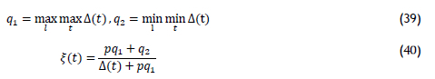
2. METHODS AND DATA
2.1. Parts selection and experiment design
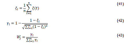
The primary focus of the experiment was to compare and discuss the applications, effects, and deficiencies of using various common forecasting methods for HR-LRU parts.
To begin the experiment, the engine driver pump (EDP) was selected as the object of study by considering the technical characteristics of HR-LRU parts maintenance. As learnt from Airbus's recommended spares list (RSPL), each aircraft requires two EDPs. The EDP's item number is 3031863-001, and its unit price is about USD 35,549. There are several reasons for choosing the EDP: (1 ) the EDP is rotable, and the aircraft cannot take off without it; (2) the EDP's mean time between unscheduled removals (MTBUR) is between 25,000 h and 35,000 h. This time is in the middle of the MTBUR of most LRUs, which has great representative significance. The average leading times for LRUs are two to four weeks, and the EDP's supplier leading time is less than ten days; (3) the EDP is required in multiple locations on a single aircraft. Large or small airlines all carry out inventory management for EDPs; (4) its high price; (5) the hydraulic brake valve and wing antiicing valve can also be selected under the same criteria. However, the EDP is a critical part of the engine, which is makes it more significant for any airplane. According to these characteristics, the EDP can replace most HR-LRU parts. By providing hydraulic power, EDPs can drive various systems on the airplane, including the rudder system, the brake system, and the retractable landing gear system.
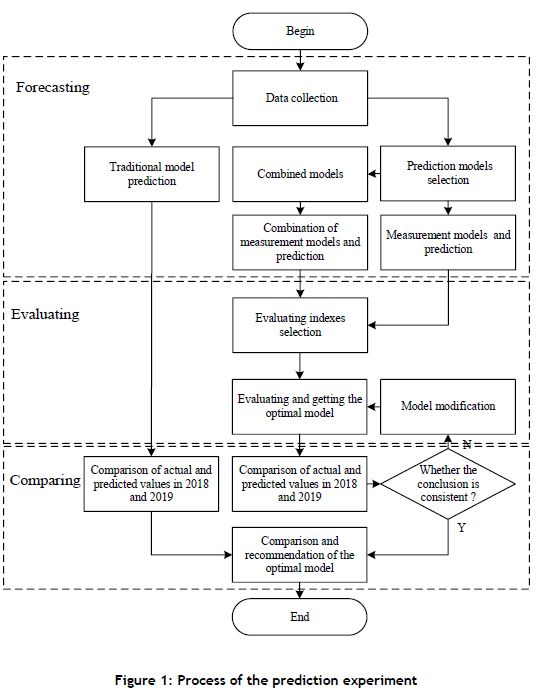
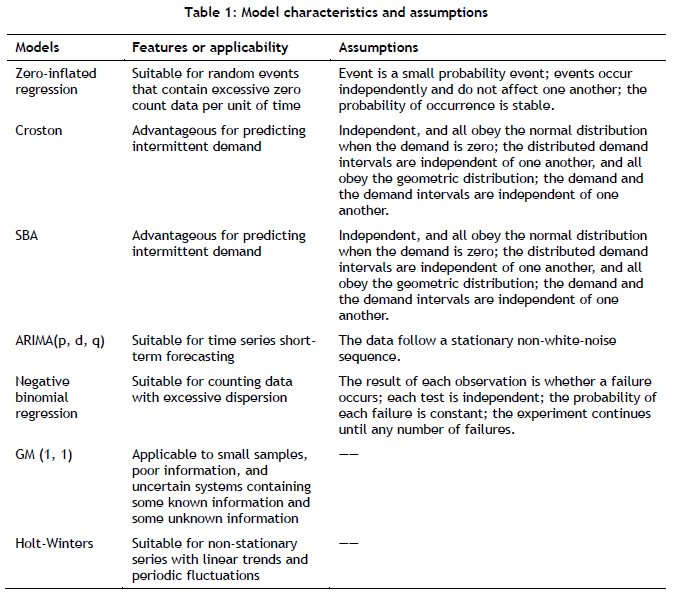
In this experiment, we introduced seven time-series prediction models for EDPs based on the literature review. Table 1 shows the features, applicability, and assumptions of these seven models. The experiment was specifically designed in three stages: forecasting, evaluating, and comparing. The forecasting stage contained three steps: using the traditional model, using seven single models, and using combined models. Five indexes were selected to evaluate the effects of the single models and the combined models. The model predictions were also compared with the actual failures that occurred during 2018 and 2019.
The whole experiment was designed to acquire an optimal prediction model for HR-LRU parts forecasting, as shown in Figure 1.
2.2. Forecasting models
2.2.1. Traditional model
The traditional forecasting method requires six sets of data, including the aircraft's flight hours, scale, turnaround time, and MTBUR. Calculations for the recommended number of HR-LRU parts can be based on Gaussian or Poisson distribution analyses.
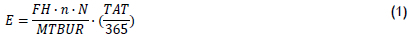
Equation (1) can be used to calculate the HR-LRU parts' demand expectation, E:
In Equation (1), FH is the number of annual flight hours, N is the number of aircraft in the fleet, n represents the quantity of parts per aircraft (QPA), MTBUR is the average unplanned replacement interval, and TAT represents the turnover time.
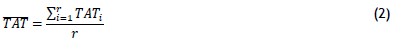
If the turnover time of the HR-LRU parts fluctuates normally, the average turnover time can be used to replace the turnover time. When a certain type of HR-LRU part has r repairing records, the turnaround time, TATt(i = 1,2, ...,r),for each repair can be expressed by Equation (2):
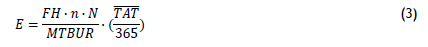
Then the HR-LRU parts' demand expectation,r, can be calculated using Equation (3):
Using the demand expectation E, the Gaussian or the Poisson distribution can be used to calculate the recommended purchase quantity, m, for HR-LRU parts according to Equation (4):
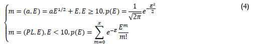
In Equation (4), PL represents the required flight guaranteed rate.
2.2.2. Measurement models
This section describes the principles and calculation steps for each model.
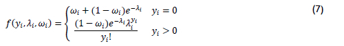
Zero-inflated Poisson regression model
The zero-inflated Poisson regression model (ZIP model) [32] is usually used to predict data types for which the proportion of zero data far exceeds other values. Its basic principle is to use a mixed calculation of the distributed Bernoulli distribution and the ordinary counting distribution, as expressed in Equation (5):

In Equation (5), ω represents the expansivity, which satisfies 0< ω < 1, and f(yt) is the distribution function.
Let a random event, , represent an HR-LRU part failure. The Poisson distribution calculates the number of random events that occur per unit of time, and assigns them as the number of HR-LRU part failures. Thus, the Poisson distribution can represent the distribution of HR-LRU part failures per unit time, and can be expressed using Equation (6):

In Equation (6), λi is the number of failures in the ith month, λi is the Poisson parameter, \i is the expectation parameter, δ2is the variance parameter, E(Y) = μ=λu and Var(Y) = δ2 = λt.
When f(yi) in Equation (6) is calculated using the Poisson distribution, the zero-inflated regression model is expressed using Equation (7):
Croston model
Croston found that, if calculations were performed at a fixed time interval, inventory predictions were equal to twice the actual demand that would be generated. This is caused by intermittent demand. Croston proposed a model, called the Croston model [33], for intermittent demand based on exponential smoothing.
If the demand, μi, is in the period, p, then the demand, Yt, can be expressed using Equation (8):

In Equation (8), n = 1,2, ...,P > 1.
The demand forecast value in each demand cycle, E(Yt), can then be calculated using Equation (9):

In Equation (9), a is the smoothing index, and it satisfies 0 < a < 1.
The Croston model assumes that the demand and the demand arrival time interval follow random distributions, and it introduces the time interval and demand distribution on this basis. The separate average time interval from average demand and the discontinuous sequence are divided into two subsets. Simple exponential smoothing is used to predict the two sub-sequences separately, as shown in Equations (10) and (11):
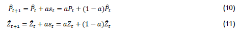
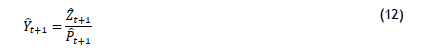
In Equations (10) and (11 ), et is the forecast error for period t, P is the demand interval after exponential smoothing, and Z£ is the demand after exponential smoothing. Then the demand forecast for the next period can be calculated using Equation (12):
SBA model
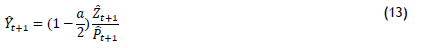
Syntetos believed that the prediction results of the Croston model were not unbiased estimates, and that the results should be adjusted. Therefore, the SBA model [34] was proposed. The SBA model uses the expression in Equation (13) to calculate the demand forecast:
ARIMA (p, d, q) model
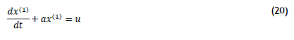
The core principle of the ARIMA time series model [35] is based on fixed time balanced series data or non-stationary time series data. It reveals the laws that exist between target variables and time changes, and uses past and present laws as well as historical data to predict the situation at a future point in time. The ARIMA (p, d, q) model was used to develop a failure prediction model based on the number of historical failures of HR-LRU parts. Assuming that an HR-LRU part's failure time is Yt, a new time series, Xt, can be obtained, as expressed in Equation (14):
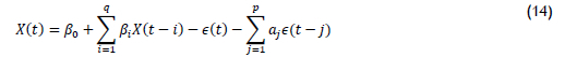
In Equation (14), p and q are the autoregressive order and the moving average order respectively, βi and ãj are the parameters, and e(t) is the white-noise sequence.
Negative binomial regression model
Many scholars believe that, when the average value and variance of a data set are not equal, or when zero-point data appear too many times, the negative binomial regression model can better fit the over-dispersed data than the Poisson distribution regression model. Negative binomial regression [36] is often used to predict the probability of a failure, accident, or illness. The probability function of this model is given in Equation (15):
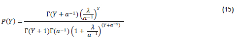
In Equation (15), μ is the overall parameter, a is the discrete parameter, and Y = 0,1,2,... . As for the Poisson regression model, Bt is the regression coefficient and λ is the exponential function of the independent variable, which can be calculated using Equation (16):

GM (1, 1) model
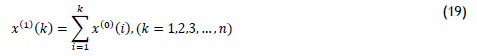
The GM (1, 1) model, also known as the grey prediction model [37], is the most common grey model. This model accumulates data to weaken the volatility caused by discrete data. Its original data sequence is given in Equation (17):

Equation (18) shows the accumulation sequence generated after accumulation:

The sequence generated by accumulation is:
The cumulative generating sequence can be used to establish cumulative generating linear differential equations, as shown in Equation (20):
The grey predicted value of the cumulative generated sequence for Equation (20) can be obtained using Equation (21):

In Equation (21 ), a and u are model parameters.
Holt-Winters model
The Holt-Winters model [6] is essentially the third exponential smoothing based on the second exponential smoothing value. Its primary purpose is to find the most suitable smoothing coefficient and to improve prediction accuracy. The fitting effect of this model is better than that of the quadratic exponential smoothing method. The Holt-Winters model is also applicable to solving all problems involving time series.
S£(1),S(2),and S(3) respectively represent the first, second, and third smoothing values at time t . yt represents the actual time series data at time t. The exponential smoothing values can be calculated using Equation (22):
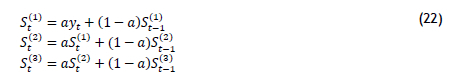
In Equation (22), a is the smoothing factor, and its value ranges between 0 and 1.
In Equations (23)-(26), at, bt, and ct are the forecast parameters of the time period, t; m is the number of forecast periods; and Ft+m is the demand value in the future m period.
2.2.3. Combined models
A weighted average of the above seven single models was conducted to form new combined forecasting models. Four common combined models were selected: the error reciprocal variable weight combination, the entropy method, the grey correlation method, and the induced ordered weighted averaging (IOWA) operator.
Error reciprocal variable weight combination
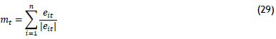
An error reciprocal variable weight combination was proposed to overcome the shortcomings of the weighted coefficient. If the single predication over-fitted, it could cause even larger errors in the combined predictions [38, 39].
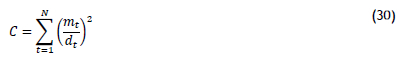
eit = (yt - ý;t)2 is the square of the prediction error of the ith method at time t. The weighting coefficient of the ith method at time t can be calculated using Equation (27):
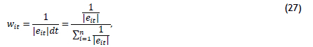
where i = 1,2, ...,n and t = 1,2, ...,N.
The coefficient vector is given as:
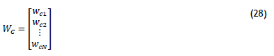
By substituting Equation (28) into Equation (27), the sum of squared errors in the error reciprocal variable weight combination forecast was obtained:
Entropy method
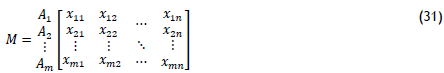
The concept of entropy is derived from thermodynamics, and is used to measure the uncertainty of a system's state. The entropy method is now commonly used to evaluate the information utility in each plan. The greater the utility value of the information, the greater the weight of the indicator.
According to the concept of entropy information, jth the multi-attribute decision matrix can be expressed using Equation (31):
Equation (32) is used to calculate the contribution of the method under the ith attribute:
Equations (33) and (34) are then used to calculate the total contribution of all methods:
The weight of each attribute is given by Equations (35) and (36):
Grey relational analysis
Grey system theory is used to analyse the grey correlation degree for each subsystem. It uses measurement methods to find numerical relationships between the subsystems in the overall system. In this research, the grey correlation method was used to determine the weights of the models.
Equation (37) expresses the dimensionless processing of data:
In Equation (37), x0(l) is the first value of the actual data set X0, xt(t) is the value of the predicted data sequence at time t, I = 0,1,2, ...,m and t = 1,2,3, ...,n.
Calculate the square difference between the dimensionless value of the actual data and the dimensionless value of the predicted data:

The correlation coefficient to transform the absolute difference data sequence is given by Equations (41) and (42):
Generally, p = 0.5 in Equation (40).
The grey correlation degree, and the weight coefficient, w,, can be calculated using Equations (41) - (43):
IOWA operator
If (ia1,y1),{a2,y2), ...,(am,ym}) are m two-dimensional arrays, then

where w =  is the weighted vector of IOWAω ,
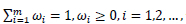 m , a - index(i) is the subscript of the largest number arranged from small to large in (a1,a2, ...,am) and IOWAω is the m-dimensional induced ordered weighted arithmetic average operator generated by (a1,a2, ...,am).
Let the number of aircraft spare part failures during a certain period be represented by yt(t = 1,2,...,n). In m combined prediction models, the prediction value of the ith combined prediction model at time t is yt(t = 1,2, ...,n). Thus, the general expression of the model is given by Equation (45):
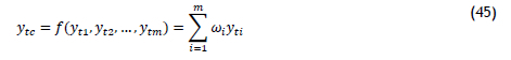
where ωt is the weight coefficient and ω1+ω2+...+ ωm = 1.
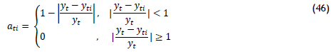
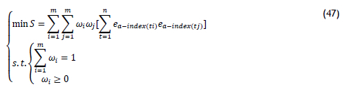
In Equation (46), ati represents the prediction accuracy of the ith single prediction model at time t, and ati is the induced value of yti. The induced value sequence of the model at time t and its corresponding predicted value form a two-dimensional array: ({at1,yt1),{at2,yt2), ...,{atm,ytm)). The induced value sequence (at1, at2,..., atm) prediction models at time t are arranged from large to small values of m. a - index(ti) is the subscript of the ith largest induced value at time t. If ea-index(ti) = yt - ya-index(ti) and the minimum sum of squared errors, S, is set as the objective function, then the combined forecasting model based on the IOWA operator can be expressed using Equation (47):
2.3. Evaluation indexes
Five evaluation indexes were selected to evaluate the effects of the single models and the combined models. The indexes are the sum of squares due to error (SSE), mean squared error (MSE), mean absolute error (MAE), symmetric mean absolute percentage error (SMAPE), and Theil inequality coefficient (TIC). The specific calculation formulas for these indexes are provided in Equations (48) - (52):
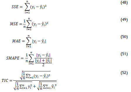
In Equations (48) - (52), yi and yi are the real observations and the predicted values respectively, and n is the number of observations.
The smaller the evaluation result, the smaller the gap between the fitted and the measured values. Small values indicate high prediction accuracy.
2.4. Data analyses
The top three airlines in China, which own the largest fleets and represent the first echelon of China's civil aviation, are Air China, China Southern Airlines, and China Eastern Airlines. In 2019, they collectively transported nearly 400 million passengers, accounting for 60% of the total passenger traffic in mainland China.
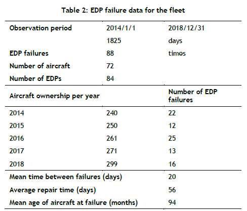
The EDP data used in this research were obtained from one of these top three airlines. The airline will be referred to as airline A due to privacy considerations. By December 31, 2019, there were 325 A320 series aircrafts within the fleet of airline A. There were 124 operating leases, 100 financial leases, and 101 self-purchased aircraft From 2014 to 2018, the airline did not experience major technological changes or large-scale model updates that made the time series data invalid. The airline had 72 aircraft with EDP failures, of which 34 were operating leases, 15 were financial leases, and 29 were self-owned aircraft. A total of 84 EDPs were removed. The average aircraft age at the time of the EDP failure was 94 months, and the average repair time was 56 days. The specific data are shown in Table 2.
The EDP failure situation for the airline's A320 series aircraft fleet from 2014 to 2018 is shown in Figure 2.
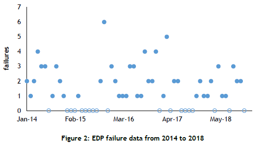
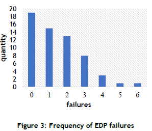
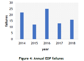
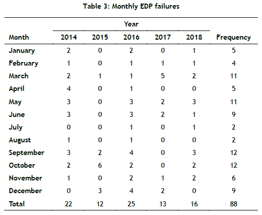
To investigate the failure situation statistically, we calculated the frequency of failures (Figure 3), the number of annual failures (Figure 4), and the number of monthly failures (Table 3). The EDP failure data indicated that the failures were intermittent [40]. In the 60 months from 2014 to 2018, there were 19 months without failures, accounting for 31.6% of the total observation time, and only one failure occurred in 15 months, accounting for 25%. On average, 1.47 EDPs failed each month. The number of failures was high in 2014 and 2016, with 22 and 25 failures respectively, accounting for 53% of the total failures. September and October had the highest number of EDP failures in all months, followed by March and May.
3. EMPIRICAL RESULTS
3.1. Traditional model results
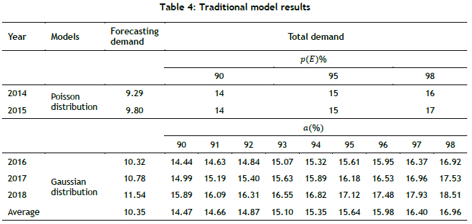
Table 4 lists the estimation results produced by the traditional model. According to the traditional model, the data from 2014 to 2015 were suitable for Poisson distribution, and the data from 2016 to 2018 were more suitable for Gaussian distribution. When the guaranteed rate was 95%, the demand forecasts for 2014 and 2015 were both 15, and the forecasts for 2016 to 2018 were 15.61, 16.18, and 17.12 respectively. The five-year average failure forecast value was 15.64. Using traditional forecasting methods, when the annual demand from 2014 to 2018 was 15, it could meet the basic requirement of the airline's guaranteed rate of 95%.
3.2. Prediction results of the measurement models
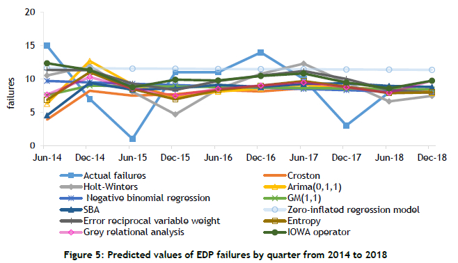
The prediction results of the measurement models and the combined models presented for each quarter from 2014 to 2018 are shown in Figure 5.
3.3. Evaluation results of the models
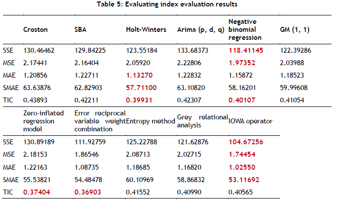
The evaluation results of the models are listed in Table 5. Under the evaluating indexes, the SSE values of the measurement models were between 118 and 134, and the SSE values of the combined model were between 104 and 126. The MSE values of most models in the measurement models were above 2, and only the MSE value of negative binomial regression was 1.97352. In the combined models, the MSE value of the error reciprocal variable weight combination was 1.86546 and the MSE of the IOWA operator was 1.74454. The MAE values of all models were between 1 and 1.23. Among the seven measurement models, the MAE values of Holt-Winters, the negative binomial regression, and GM (1, 1) were below 1.2. The values of SMAPE were between 53 and 64. The TIC values of most models were above 0.4. The TIC values of Holt-Winters, the zero-inflated regression model, and the error reciprocal variable weight combination were lower than 0.4.
3.4. Prediction results of all models
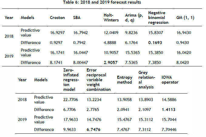
The prediction results of all models and the actual data from 2018 and 2019 are provided in Table 6. The differences between the predicted value of measurement models and the actual data in 2018 were 0.16 to 6.78, which was a large gap. The differences of the combined model were between 1.4 and 2.78. The differences between the predicted results in 2019 and the actual data were mostly between 7-8.
4. DISCUSSION
4.1. Shorter MTBF leads to a downward trend in guaranteed rate
The traditional model indicated that, when the airline's guaranteed flight rate was required to reach 95%, the total demand for EDPs was approximately 16, as shown in Table 4. In addition, when the inventory was 16, the guaranteed rate was 98% in 2014, 96% in 2015 and 2016, 94% in 2017, and 90% in 2018. For the same number of spare parts, the guaranteed rate decreased year by year. The reason for this may be a shorter
mean time between failure (MTBF), which increases the demand expectation, E , for HR-LRU parts. MTBF is a commonly used parameter to calculate the failure probability of spare parts. The reduced MTBF of HR-LRU parts has several potential causes:
1) In the past five years, maintenance personnel may have reduced maintenance capabilities and increased HR-LRU part failures for reasons such as slow updates in maintenance knowledge, few professional skills, and company layoffs.
2) The same HR-LRU parts may be used from the beginning to the end of the product's life cycle. HR-LRU part performance decreases may be due to wear, material degradation, and sudden failures.
3) HR-LRU parts are high-value and high-reliability products. They are limited by test cost and cycle time. The number of field tests and failure data are generally small. Classical mathematical statistics methods have difficulty in reflecting the actual reliability levels [41].
4) The storage environments for HR-LRU parts are demanding. In high humidity, salt sprays, or a polluted atmosphere, corrosion, deterioration, cracking, and other adverse conditions may cause the number of failures to increase. In addition, different suppliers have different manufacturing technologies and skills for fabricating HR-LRU parts, all of which may also be related to the decreasing MTBF.
4.2. Model performance according to the fitting image
Figure 5 shows the prediction results of the various models. The quarterly total failure value for the EDPs fluctuated significantly, and the difference between the maximum value and the minimum value was 15. Among all of these models, the Holt-Winters model predicted the value fluctuations best. The gap between the maximum and minimum values was the largest, which was about 8, and this model's prediction was closest to the actual value. Among the measurement models, the values fitted by the Croston model and the SBA model were similar, and the fitted value of the negative binomial regression model was close to that of the GM (1, 1). For the combined prediction models, the fitted value of the error reciprocal variable weight model was similar to that of the IOWA operator. The results of the entropy method and the grey relational analysis were approximately equal. In addition, except for the zero-inflated regression model, most of the models' predicted values fluctuated around the 7-11 range. The forecast value of the zero-inflation regression tended to be 12 and was relatively stable, and had the largest deviation from the true value.
4.3. Model performance according to the evaluating indexes
Table 5 indicates the key findings of this investigation: the Holt-Winters, the zero-inflated regression model, and the negative binomial regression models had the best prediction results of all of the measurement models. They had similar prediction accuracies under the five evaluations indexes, and their accuracies were higher than for the other models. Holt-Winters had the best results among the seven models of MAE, which were 1.13270. The negative binomial regression had the second-best effect at 1.15872. The SSE and MSE indicators of negative binomial regression were the best, which were 118.4114 and 1.97352 respectively. The SMAPE and TIC of the zero-inflated regression model were the lowest. Holt-Winters and the negative binomial regression were the second and third best respectively: Their SMAPEs were 57.71100 and 58.16201 and their TICs were 0.39931 and 0.40107 respectively. Among the four combined models, the IOWA operator performed best, and the error reciprocal variable weight model followed. Moreover, these two combined forecasting models performed better than the single models.
4.4. Comparison of actual and predicted values
The forecasting results for 2018 and 2019 also supported the above findings. According to Table 6, in the year 2018, the gap between the actual value and the prediction result from the negative binomial regression model was the smallest at only 0.1693. The error of the IOWA operator was the smallest for all the combined models at only 1.4113. For the prediction of failures in 2019, the Holt-Winters model and the reciprocal error performed best among the single models and the combined models respectively.
It was also observed that, when making predictions for EDPs, out of the single models, the Holt-Winters and the negative binomial regression models could be used. For the combined models, the IOWA operator and the error reciprocal variable weight could be selected. The comparison showed that some single models produced predictions much closer to the actual values than those of the combined models. The reason for this may be related to the weight of the single models in the forecast value for the year in the combined forecast. In addition, both the negative binomial regression model and the IOWA operator could meet the general requirements for airlines with a flight guaranteed rate of above 95% for HR-LRU parts purchasing.
4.5. Comparison with other studies
The methods or research objects adopted in this study were the same as those in some other studies[42]. Through comparison, we found some similarities and differences. Wang et al. [43] chose eight prediction models: the Poisson distribution model, the linear regression model, the AR model, the ARIMA (p,d,q) model, the automatic ARIMA model, the Holt-Winters model, the GM (1,1 ) model, and the SVR model. They used aviation spare parts data to make demand forecasts, and found the best forecasting method to be gray correlation and association rules mining. Among the eight prediction models, the support vector machine regression model performed best in December 2011 and the ARIMA (p,d,q) model outperformed other prediction models in December 2013. According to the association rules, the applicability of the automatic ARIMA model was better than other forecast models for spare parts. In our research, the Holt-Winters model had a better predictive effect than the ARIMA (p,d,q) model. The reasons may be the following. (1 ) Different research objects. Although this study and the literature selected aviation spare parts for the research, this study focused on the prediction of HR-LRU parts, while the literature did not state the types of aviation spare parts for its research objects. It is possible that the research object did not focus on a certain kind of aviation spare part, so different research objects may cause different conclusions. (2) Different evaluation criteria. This paper mainly chose the comparison of evaluation indicators to make judgements, while the literature chose gray prediction and association rules mining to make judgements. (3) Different data sources. In the literature, the authors did not state whether the source of the data was the same type of aircraft from the same fleet. This was somewhat different from the uniformity of our data sources. And the data came from 2001 to 2013, which is a long and relatively old period, which was also different from our data.
In another paper [6], the Holt-Winters method was found to be more suitable for long-term forecasting and monthly short-term forecasting by comparing 16 forecasting methods to predict heat load. Although the research objects were different, the data characteristics and research results were similar to those in this article. It can also be seen that our conclusions could be used for reference.
5. CONCLUSIONS
Based on the failure data of EDPs from 2014 to 2018, among seven single measurement models, the negative binomial regression model and the Holt-Winters model produced better predictions than all of the other models. The SSE and MAE of the negative binomial regression were the lowest at 118.41145 and 1.97352 respectively, and the Holt-Winters model's MAE was the lowest at 1.13270. Under the evaluation of SMAPE and TIC, the performances of the Holt-Winters and negative binomial regression models were also the second- and third-best among all seven measurement models. Their SMAPEs were 57.71100 and 58.16201 and their TICs were 0.39931 and 0.40107 respectively. Among the four combination models, the accuracy of the IOWA operator predictions was better than the others; the SSE was 104.672 5 and the SMAPE was 53.116 92. The reciprocal error method also produced good results. Compared with real data in 2018, the prediction errors of the negative binomial regression model and the IOWA operator model were only 0.1693 and 1.4113 respectively. In addition, the former model's results could meet 95% of the airline's guaranteed requirements, and the latter model's results could meet 97% of the actual needs of the guaranteed rate. There were eight EDP failures in 2019, and the predicted values of the Holt-Winters model and the error reciprocal variable weight combination model were closest to the actual values. The errors were 2.9057 and 6.7476 respectively.
This study's results confirm that measurement models are good choices for airline cost control. Compared with traditional models, measurement models could avoid the shortcomings of collecting diverse data. The measurement models only had to count the number of failures, making it easier for airlines to control the cost of the HR-LRU parts. One limitation of these methods, however, is the time-series data failure. In the face of occasional emergencies (such as COVID-19), major technological changes, and large-scale model updates, start-up airlines can use traditional models with data from other airline allies or competitors.
The study found that, in 2019, if calculated according to the 95% guaranteed rate, the traditional model needed to prepare 16 EDPs, while the Holt-Winters model required 11. The difference between the two calculation results was five EDPs. The purchase price of five EDPs is USD 177,745. In the A320 fleet, there are more than 500 aircraft spare parts with a price of more than USD 10,000 and an essentiality code (ESS)=2. When there are similar redundant purchases, the redundant expenditure can be as high as USD 300 million, based on the average purchase price. It was found that the use of higher-precision forecasting methods had considerable effects on airline cost control.
Regarding the prediction results, the prediction values of the traditional model and of the measurement models were higher than the actual value in 2019. There are two primary reasons for this. (1) The true value of failures in 2019 may have been significantly affected by the age of the aircraft in the airline's fleet. The aircraft age factor was not considered in the above models. (2) The airlines' aircraft maintenance capabilities may have been greatly improved in 2019, increasing the interval between the failures of EDPs currently operating in the aircraft. These specific reasons, among others, should be explored in the future.
The concern about the experimental findings was that the features of the HR-LRU parts were different. As the complexity of aircraft systems increases, the number of aircraft HR-LRUs increases. The intricate cross-linking relationship between them complicates the failure of HR-LRU parts. Whether the characteristics of EDP can replace all LRU parts, and whether EDP failure data can be used to predict the failure of LRU parts, is still controversial. This is worth further discussion. Owing to the outbreak of COVID-19, it is also difficult to obtain valid data to verify. In addition, emerging technologies, such as artificial intelligence, the big data industry, and the internet, might prove to be promising areas for future research. More alternative methods could also be tried. In future work, we plan to use these emerging technologies based on measurement models, combined with the predictive maintenance data of airlines, to improve the accuracy of HR-LRU part forecasting, and to use data from other fleets or time periods to validate our conclusions.
ACKNOWLEDGMENTS
This work was supported by the Tianjin Municipal Education Commission Scientific Research Project (2020SK046) and the Tianjin Research Innovation Project for Postgraduate Students (2021YJSS105). The authors are grateful to the airline for providing the data. We thank LetPub (www.letpub.com) for linguistic assistance and a pre-submission expert review.
REFERENCES
[1] Backhaus, J. 1980. The Pareto principle. Analyse und Kritik, 2(2), pp. 146-171. [ Links ]
[2] Prestwich, S. D., Tarim, S. A., & Rossi, R. 2021. Intermittency and obsolescence: A Croston method with linear decay. International Journal of Forecasting, 37(2), pp. 708-715. [ Links ]
[3] Lin, L., Chen, X., & Zhong, S. 2016. A new approach of forecasting intermittent demand for spare parts. Journal of Harbin Institute of Technology, 48(01 ), pp. 40-45. [ Links ]
[4] Wei, Z., & He, J. M. 2013. Generalized GM (1, 1) model and its application in forecasting of fuel production. Applied Mathematical Modelling, 37(9), pp. 6234-6243. [ Links ]
[5] Mohanad S. Al-Musaylh, Ravinesh C. Deo, Jan F., & Yan L.. 2018. Short-term electricity demand forecasting with MARS, SVR and ARIMA models using aggregated demand data in Queensland, Australia. Advanced Engineering Informatics, 35, pp. 1-16. [ Links ]
[6] Tratar, L. F., & Strmcnik, E. 2016. The comparison of Holt-Winters method and multiple regression method: A case study. Energy, 109, pp. 266-276. [ Links ]
[7] Peng, Y., Zhou, L., Wang, S., & Zeng, Q. 2018. Spare parts allocation optimization for extremely low duty equipment storage and use stage. Systems Engineering and Electronics, 40(10), pp. 22702275. [ Links ]
[8] Li, P., Yuan, H., Cao, Z., & Zhang, H. 2016. Quantitative method of dynamic fault tree analysis for imperfect coverage system. Journal of Beijing University of Aeronautics and Astronautics, 42(09), pp. 1986-1991. [ Links ]
[9] Feng, Y., Cheng, L. U., Xue, X., & Yongkai, L. I. 2018. Single-echelon initial inventory optimal allocation for civil aircraft spare parts with importance degree. Journal of South China University of Technology (Natural Science Edition), 46(09), pp. 140-148. [ Links ]
[10] Mobarakeh, N. A., Shahzad, M. K., Baboli, A., & Tonadre, R. 2017. improved forecasts for uncertain and unpredictable spare parts demand in business aircrafts with bootstrap method. Ifac Papersonline, 50(1), pp. 15241-15246. [ Links ]
[11] Zhang, X., Wang, N., Xiao, B., & Lin, M. A. 2019. Availability modeling of parallel-series system under influence of spare parts and maintenance turnover. Systems Engineering and Electronics, 41 (01 ), pp. 223-228. [ Links ]
[12] Feng, Y., Lu, C., Xue, X., & Liu, Y. 2018. Multi-echelon inventory allocation of civil aircraft spare parts considering maintenance ratio. Xibei Gongye Daxue Xuebao/Journal of Northwestern Polytechnical University, 36(3), pp. 582-589. [ Links ]
[13] Pinçe, C., Turrini, L., & Meissner, J. 2021. Intermittent demand forecasting for spare parts: A critical review. Omega, 105(1), 102513. [ Links ]
[14] Guo, F., Diao, J., Zhao, Q., Wang, D., & Sun, Q. 2017. A double-level combination approach for demand forecasting of repairable airplane spare parts based on turnover data. Computers & Industrial Engineering, 110, pp. 92-108. [ Links ]
[15] Romeijnders, W., Teunter, R., & Van Jaarsveld, W. 2012. A two-step method for forecasting spare parts demand using information on component repairs. European Journal of Operational Research, 220(2), pp. 386-393. [ Links ]
[16] Li, B., Ding, J., Yin, Z., Li,K., Zhao, X. & Zhang, L. 2020. Optimized neural network combined model based on the induced ordered weighted averaging operator for vegetable price forecasting. Expert Systems with Applications, 168, 114232. [ Links ]
[17] Li, H., Wang, J., Lu, H., & Guo, Z. 2018. Research and application of a combined model based on variable weight for short term wind speed forecasting. Renewable Energy, 116, pp. 669-684. [ Links ]
[18] Moreira, M. O., Balestrassi, P. P., Paiva, A. P., Ribeiro, P. F., & Bonatto, B. D. 2021. Design of experiments using artificial neural network ensemble for photovoltaic generation forecasting. Renewable and Sustainable Energy Reviews, 135, 110450. [ Links ]
[19] Wang, J., Zhou, H., Hong, T., Li, X., & Wang, S. 2020. A multi-granularity heterogeneous combination approach to crude oil price forecasting. Energy Economics, 91, 104790. [ Links ]
[20] Wang, L., Wang, Z. G., Qu, H., & Liu, S. 2018. Optimal forecast combination based on neural networks for time series forecasting. Applied Soft Computing, 66, pp. 1-17. [ Links ]
[21] Long, H., & Yan, G. 2016. Forecasting import and export volume with a combined model based on wavelet filtering. International Journal of Wavelets Multiresolution & Information Processing, 14(03), 1650018. [ Links ]
[22] Shan, Y., Fu, Q., Geng, X., & Zhu, C. 2016. Combined forecasting of photovoltaic power generation in microgrid based on the improved BP-SVM-ELM and SOM-LSF with particalization. Proceedings of the CSEE, 36(12), pp. 3334-3342. [ Links ]
[23] Zheng, A., Liu, W., & Zhao, F. 2010. Double trends time series forecasting using a combined ARIMA and GMDH model. Paper presented at the Proceedings of 2010 Chinese Control and Decision Conference. pp. 1820-1824. [ Links ]
[24] Zhang, G.P. 2003. Time series forecasting using a hybrid ARIMA and neural network model. Neurocomputing, 50, pp. 159-175. [ Links ]
[25] Wei, Y., Bai, L., Yang, K., & Wei, G. 2020. Are industry-level indicators more helpful to forecast industrial stock volatility? Evidence from Chinese manufacturing purchasing managers index. Journal of Forecasting, 40(1), pp. 17-39. [ Links ]
[26] Yang, S. X., Cao, Y., Liu, D., & Huang, C. F. 2011. RS-SVM forecasting model and power supply-demand forecast. Journal of Central South University of Technology, 018(006), pp. 2074-2079. [ Links ]
[27] Jin, F., Li, Y., Sun, S., & Li, H. 2020. Forecasting air passenger demand with a new hybrid ensemble approach. Journal of Air Transport Management, 83, 101744. [ Links ]
[28] Wang, H., Sun, J., & Wang, W. 2018. Photovoltaic power forecasting based on EEMD and a variable-weight combination forecasting model. Sustainability, 10(8), 2627. [ Links ]
[29] Qu, L. L., & Yan, C. 2016. An adaptive time-variable weight combination forecasting method for time series. 2006 International Conference on Management Science and Engineering , pp. 318-323. [ Links ]
[30] Li, W. Q., & Li, C. 2018. A combination model with variable weight optimization for short-term electrical load forecasting. Energy, 164, pp. 575-593. [ Links ]
[31] Liu, J., Wang, S., Wei, N., Chen, X., Xie, H., & Wang, J. 2021. Natural gas consumption forecasting: A discussion on forecasting history and future challenges. Journal of Natural Gas Science and Engineering, 90, 103930. [ Links ]
[32] Kim, K.-M. 2003. An application to multivariate zero-inflated poisson regression model. Journal of the Korean Data & Information Science Sociaty, 14(1 ), pp. 45-53. [ Links ]
[33] Croston, J. D. 1972. Forecasting and stock control for intermittent demands. Journal of the Operational Research Society, 23(3), pp. 289-303. [ Links ]
[34] Syntetos, M., Boylan, J. E., & Croston, J. D. 2005. On the categorization of demand patterns. Journal of the Operational Research Society, 56(5), pp. 495-503. [ Links ]
[35] Newbold, P. 2010. ARIMA model building and the time series analysis approach to forecasting. Journal of Forecasting, 2(1 ), pp. 23-35. [ Links ]
[36] Chang, L. Y. 2005. Analysis of freeway accident frequencies: Negative binomial regression versus artificial neural network. Safety Science, 43(8), pp. 541-557. [ Links ]
[37] Wang, Z.-X., Li, D.-D., & Zheng, H.-H. 2020. Model comparison of GM(1,1) and DGM(1,1) based on Monte-Carlo simulation. Physica A: Statistical Mechanics and its Applications, 542, 123341. [ Links ]
[38] Liu, Y. 2000. Overfitting and forecasting: Linear versus non-linear time series models. ISU General Staff Papers.Iowa State University. [ Links ]
[39] Radchenko, P., Vasnev, A. L., & Wang, W. 2020. Too similar to combine? On negative weights in forecast combination. International Journal of Forecasting, 39(1), pp. 18-35. [ Links ]
[40] Regattieri, A., Gamberi, M., Gamberini, R., & Manzini, R. 2005. Managing lumpy demand for aircraft spare parts. Journal of Air Transport Management, 11(6), pp. 426-431. [ Links ]
[41] Dong, H., Wan, L., Yang, Y., & Yi, X. 2017. Bayesian assessment on MTBF of aero-engine. Hangkong Dongli Xuebao/Journal of Aerospace Power, 32(8), pp. 1978-1983. [ Links ]
[42] Cao, Y., Liu, Y., & Shen, D. 2022. Demand Forecast Model Comparison of Airline LRU Parts. Industrial Engineering Journal(in Chinses), 25(6), pp. 101-109. [ Links ]
[43] Wang, J., Pan, X., Wang, L., & Wei, W. 2018. Method of spare parts prediction models evaluation based on grey comprehensive correlation degree and association rules mining: A case study in aviation. Mathematical Problems in Engineering, 2018, pp. 1-10. [ Links ]
Submitted by authors 14 Apr 2022
Accepted for publication 5 Sep 2022
Available online 14 Dec 2022
* Corresponding author: dyshen@cauc.edu.cn
ORCID® identifiers
Y. Cao: 0000-0003-0505-8802
Y. Liu: 0000-0002-2666-5823
D. Shen: 0000-0002-7937-7198

