SPECIAL EDITION

 

Development of emission intensity factors for a South African road-freight logistics service provider

 

 

M.J. du Plessis^*; J. van Eeden; M. Botha

Department of Industrial Engineering, Stellenbosch University, South Africa

 

 

---

ABSTRACT

The Global Logistics Emissions Council (GLEC) framework developed logistics emission factors to be used uniformly in North America and Europe. It included an approximation for African countries; however, actual South African emissions were not accurately reflected. Therefore, in this study, carbon emissions factors were calculated using calculated tonne-kilometres and the energy-based methodology. The authors obtained several datasets from a logistics service provider (LSP) consisting of vehicle routes, refuelling data, and freight load data. The project developed factors for each individual trip, for similar repetitive trips, and for the entire data set. These different sets of factors were developed to allow the use of different emission calculation and reporting standards. The LSP could use these emission intensity factors to estimate carbon emissions using the activity-based approach, report emissions according to legislation, and predict how much carbon emissions would be emitted to move a customer's shipment.

---

OPSOMMING

Die Global Logistics Emissions Council (GLEC) raamwerk het logistieke emissiefaktore ontwikkel vir eenvormige gebruik in Noord-Amerika en Europa. Alhoewel dit 'n benaderde skatting vir Afrika-lande insluit, word die werklike Suid-Afrikaanse emissies egter nie akkuraat weerspieel nie. In hierdie studie word koolstofvrystellingsfaktore bereken deur die gebruik van berekende ton-kilometer sowel as energie-gebaseerde metodologie. Die outeurs het verskeie datastelle van 'n logistieke diensverskaffer verkry wat bestaan uit die roetes gebruik deur hul voertuie, brandstofdata sowel as vrag data. Die projek het faktore ontwikkel vir individuele vragverskuiwings, vir soortgelyke herhalende vragte, en vir die datastel in sy geheel. Hierdie verskillende stelle faktore is ontwikkel om die gebruik van verskillende emissieberekeninge en verslagdoeningstandaarde moontlik te maak. Die logistieke diensverskaffer kan nou hierdie emissie-intensiteitsfaktore gebruik om koolstofvrystellings te skat deur die aktiwiteitsgebaseerde benadering te gebruik. Hierdie emissie-intensiteitsfaktore kan ook gebruik word om emissies te rapporteer soos vereis word deur wetgewing, en om te voorspel hoeveel koolstof vrygestel sal word om 'n klient se vrag te verskuif.

---

 

 

1. INTRODUCTION

Terms such as 'greenhouse gases' (GHGs), 'emissions', and 'carbon footprint' have become common buzzwords in modern society [1], [2]. Owing to increased pressure, governments, organisations, and individuals often use these terms to create an illusion of environmental sustainability [2], [3]. In most cases, unfortunately, this is only done to advance economic or political interests [4]. Despite a lack of understanding of the sources or size of emissions, ambitious emission reduction goals or targets are still set. Ideally, before organisations set emission reduction targets, a good starting point would be to quantify how carbon-intensive everyday business activities are. An analysis would enable organisations to understand how they produce emissions and allow future comparisons to measure progress.

This is particularly relevant in the road-freight industry, since LSPs often do not know the quantity of emissions when transporting a shipment. In addition, clients increasingly ask transporters how much is emitted as a result of the transport of their cargo. However, the field of allocating freight transport emissions is still in its infancy [5]. This is evident from research done by Du Plessis et al. [6] and the Smart Freight Centre [7] that shows the lack of sector-specific guidance to aid stakeholders in determining distributional emissions.

Many companies in the road-freight sector face the same challenge: how much is emitted on average when moving a tonne of freight one kilometre? This factor is known as the 'emission intensity factor' (EIF). Although EIFs are available in the literature [7], [8], [9], the accuracy and relevance of these suggested factors to the South African road-freight sector is questionable. Accurately calculating the emissions of transport activities is essential for any road-freight company to understand how its actions and decisions create emissions. This would allow LSPs to compare alternative transportation scenarios potentially to decrease emissions.

Thus this paper establishes an EIF for a large road-freight company, Company X, that operates in over 20 countries and employs over 10 000 people. The developed EIF is specifically for the tanker division, which transports bulk liquids in South Africa. This enables Company X to determine how much emissions is emitted by a typical shipment, and allows internal benchmarking to gauge its progress in reducing emissions.

 

2. LITERATURE REVIEW

This section briefly reviews the literature by discussing the importance of emission reduction and the associated pressure on organisations. Section 2.2 provides an overview and profile of South Africa's road-freight emissions, while Section 2.3 explains how to quantify LSPs' emissions and the problems associated with doing this accurately. The final section discusses the available EIFs found in the literature.

2.1. The importance of reducing emissions

The global community has pledged to reduce GHG emissions on several occasions. The most notable are the 1992 United Nations Framework Convention on Climate Change (UNFCCC), the 1997 Kyoto Protocol, and, more recently, the Paris Agreement of 2015. According to the Intergovernmental Panel on Climate Change (IPCC) [10], global GHG emissions must peak by 2025 and then reduce by 43% in 2030 if a 1.5 °C temperature increase is going to be achieved. In response to these global agreements, South Africa agreed to reduce emissions by 42% by 2025 [11]. In addition, the South African Government signed into law the Carbon Tax Act (Act No. 15 of 2019), which imposes a tax of ZAR 120 per tonne of CO2e emitted. This amount was increased to ZAR 144 per tonne of CO2e for the year 2022, whereafter the value will increase by the consumer price inflation (CPI) each year [12]. The Air Quality Act (Act No. 39 of 2004) also requires organisations above an annual emission threshold of 0.1 Mt CO2e to report their emissions to the South African Greenhouse Gas Emissions Reporting System (SAGERS). This forces organisations to calculate and report their total emissions (Scope 1 and Scope 2 emissions) according to the GHG Protocol Corporate Accounting and Reporting Standard [13]. In addition, customers put pressure on companies to reduce their emissions, or else they will take their business elsewhere [14]. It is clear that organisations have both a legal requirement and a corporate responsibility to transition to a decarbonised economy that uses renewable energy, low-carbon technology, and less fossil fuel. Adapting to an environmentally sustainable business model is a definite prerequisite to remain relevant and competitive.

2.2. Road-freight emissions

According to Ajhum, Merven, Stone and Caetano [15] and the South African Department of Transport [16], the entire transport sector in South Africa emits around 60 MtCO2e per annum. This represents nearly 14% of South Africa's total emissions [17]. Road freight accounts for 90.0% to 91.2% of the transport sector's emissions [16], [17]. The proportion of road-freight emissions is expected to increase even further, since Transnet Freight Rail (TFR) can no longer provide an adequate rail service - as is evident from the recently declared force majeure on several coal contracts [18]. Road transport is and will become increasingly important for any freight movement in South Africa.

Authors such as Ahjum et al. [15] predict that electric, hydrogen, biofuel, and natural gas vehicles will become a reality in a future South Africa. However, authors such as Mckinnon [5] state that the transport sector is one of the most challenging industries to decarbonise, since it relies heavily on fossil fuels. Until alternative fuels and vehicles become a reality and a shift occurs, heavy-duty diesel trucks will continue to transport the vast majority of freight in South Africa and globally. Authors such as Kamdar [19] estimate that there are up to 350 000 freight trucks on South Africa's roads alone. Thus a better understanding of how road transport vehicles produce emissions when transporting cargo is essential.

Various factors - such as the vehicle's speed, aerodynamics, engine and powertrain technology, driver behaviour, waiting and idle time, operational efficiency and route planning, load factor, empty running or potential backhaul, service interval, tyre pressure, and use of low-resistance tyres - affect the emissions of a transport activity. However, before a micro bottom-up analysis is done to determine the impact of these individual factors, the current system's emissions should be known. This requires a top-down assessment to identify the status quo, which is the purpose of this paper.

2.3. Quantifying the emissions of road transport

There are two possible methods to calculate the emissions of all freight transport activities: the energy-based approach and the activity-based approach [7], [8]. Since most emissions from road-freight transport are energy-related, the first method uses the amount of fuel used (€) and an emission factor (kg CO2e/l) to convert the energy usage to emissions (kg CO2e). This is known as the energy-based approach, since the actual amount of energy consumed during each trip is used to calculate the emissions. The activity-based method estimates the emissions when the actual energy consumption (l of fuel used per trip) is unavailable. This method uses an EIF (kg CO2e/t-km), the shipment weight (t), and the distance (km) to estimate the emissions (kg CO2e) of a shipment. A vehicle's fuel usage is replaced, therefore, with an average factor that estimates how much fuel is used to move one tonne of freight a kilometre.

The energy-based approach is always more accurate than the activity-based approach. The actual fuel consumption of a trip accounts for vehicle efficiency, vehicle age, trailer configuration, load factor, cargo type, empty running, driver habits, route travelled, traffic conditions or congestion, waiting or idle time, and weather conditions. The activity-based method, however, assumes that the chosen EIF variables are similar to the shipment being calculated, which is not always true. It is evident that there is a need for various appropriate and accurate EIFs to be used in the activity-based method.

Despite the shortcomings and apparent flaws of the activity-based method, it is still a valuable method for estimating emissions, once an appropriate EIF is available. The method could increase in popularity because of its ease of use and its ability to cover data shortcomings such as fuel usage or detailed payload, which only the LSP knows.

2.4. EIF for road transport

Even though road transport is important, no research has assessed the carbon intensity of the mode in South Africa. In addition, there is little peer-reviewed international research about road freight's EIF in the public domain. However, the Global Logistics Emissions Council (GLEC) framework [7] suggests a comprehensive set of EIFs for different sizes of road transport vehicle. These EIFs are conservative, and apparently overestimate the emissions in most cases. The suggested factors account for the type of load transported, the load factor, and the vehicle's percentage of empty running. Table 1 indicates the EIF for a large articulated truck (gross vehicle mass [GVM] less than 60 t), which is comparable to that of Company X, analysed in this research. Although the factors are for Europe and South America, the Smart Freight Centre (SFC) [7] states that the European and South American EIFs can be used for Africa if they are increased by 22%, as shown in Table 1. The GLEC's proposed upliftment by 22% is based on the extrapolation of an International Council on Clean Transportation dataset. However, the present authors question the accuracy of this 'blanket' upliftment between different regions. Despite its limitations, the suggested EIF is a good starting point for Company X to estimate the scale or size of emissions for this type of truck configuration - although it should be noted that this is not specific to a tanker truck.

 

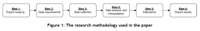
3. RESEARCH METHODOLOGY

The methodology used in this study is divided into six steps, as displayed in Figure 1. Each of the steps is discussed in more detail below.

3.1. Project scoping

This study uses the principles, boundaries, and methods for transport service analysis stated in the European Standard EN 16258:2012 [20], which is used to calculate the EIF of individual trips. In addition, the United States Environmental Protection Agency (US EPA) SmartWay methodology [9] is used to calculate the overall average EIF of the entire truck fleet. Both methodologies ([20], [9]) are used and accepted in the GLEC framework, and so are used in this paper.

Reference must be made to the allocation of the emissions of milk-run deliveries, since a different method is used. Milk runs are different because the shortest theoretical distance between the origin and the destination is used to allocate the emissions. This differs from [9] and [20], which would use the travel distances between successive delivery locations. This means that the emission allocation of milk runs is independent of the actual distance driven by the vehicle. Refer to the World Business Council for Sustainable Development (WBCSD) and the World Resources Institute (WRI) [21] (pp 63-64) for a detailed example.

This paper analyses the cradle-to-grave (also known as the 'well-to-wheel') emissions from the physical distribution or transportation of bulk liquid by an on-road truck. The emissions and the EIF are stated as a carbon dioxide equivalent (CO2e). All other emissions from to the construction, maintenance, and disposal of infrastructure, vehicles, or consumables are outside the project's scope.

The project focused on Volvo FH440 truck tractors pulling tri-axle food-grade tankers with a maximum capacity payload of 36 tonnes. Figure 2 is a diagram of the truck-and-trailer combination analysed in this paper. Eight representative trucks from Company X's fleet were selected, and all trip movements for a three-month period were analysed.

3.2. Data requirements

The following data values were required for each trip, and were collected or derived from Company X's data:

■ Departure date and time;

■ Arrival date and time;

■ Pickup location;

■ Delivery location;

■ Empty running distance/percentage;

■ Load factor;

■ Total trip distance;

■ Amount of diesel fuel used during the trip.

Another important data value that is needed is the fuel emission factor (kg CO2e/l) of diesel fuel. Company X requested their fuel provider, a multinational South African fuel company, to provide the project with a country-specific factor for diesel fuel. The fuel company acknowledged the importance of such a factor, but stated that there were no immediate foreseeable plans to establish such a factor. Since a country-specific fuel emission factor could not be obtained for this project, 3.11 kg CO2e/l was used. This value is the average of the European and North American factors as proposed in the GLEC framework [7].

3.3. Data collection

Despite the size and technological advancement of Company X's business processes, collecting the required data presented a number of challenges. Several data systems, each from a different department in Company X, were integrated to create a complete list. These were the transport management system (TMS), the vehicle telematics system, the fuel management system, the asset register, the client base file, and the delivery files. These different systems were integrated into a single Excel file that could derive or calculate all the required fields, as stated in Section 3.2.

3.4. Data analysis and interpretation

The details of the data analysis and interpretation are discussed in Section 4, given its importance.

3.5. Calculation

In order to determine the EIF of a transport activity, the equations given in this section were used. Note that it is a prerequisite that the data be in the correct format.

Emission intensity factor

To calculate the EIF of a single shipment, Equation (1) was used:

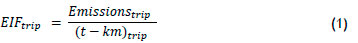
where EIF_trip is the emission intensity factor (kg CO₂e/t-km), Emissions_trip is the total CO₂e emissions (kg) emitted during the trip based on actual fuel consumed, and (t-km)trip is the tonne-kilometre value of the trip. The (t-km)_trip value in milk runs is the sum of all origin-destination pairs' tonne-km values, as stated in Equation (3).

Total emissions

In order to calculate the emissions for each trip, Equation (2) was used:

where Emissionstrip is the total amount of CO2e emissions (kg) emitted during the transport activity, Fuel_used is the total amount of diesel fuel in litres (l) used during the trip, and Emission Factor is the fuel emission factor for diesel fuel (3.11 kg CO₂e/l).

Tonne-kilometre

The tonne-kilometre value for each trip can be calculated as shown in Equation (3):

where (t - km)trip is the tonne-kilometre value, Weightcargo is the weight (t) of cargo moved, and Distance_loaded is the road distance travelled (km) between the collection and delivery points of the shipment. Note that, in milk runs, Weightcargo refers to the weight of cargo delivered to the specific delivery location, while Distanceloaded refers to the shortest theoretical road distance between the origin and the delivery destination.

Load factor

The load factor is a ratio that describes how heavily a transport vehicle is loaded. For each trip, this can be calculated using Equation (4):

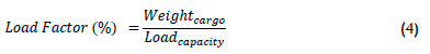
where Load Factor (%) is the load factor of the trip, Weightcargo is the weight (t) of the cargo moved, and Load_capacity is the maximum payload capacity (36 t) of the transport vehicle. In milk runs, Weightcargo is the weight (t) of cargo initially loaded onto the vehicle.

Empty running

The empty running of a transport vehicle is a ratio that indicates what proportion of travelled distance a vehicle is not carrying cargo. This is also referred to as 'lost' kilometres. For each trip, this can be calculated using Equation (5):

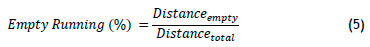
where Empty Running (%) is the empty running for the trip, Distanceempty is the total distance travelled empty (km) during the trip, and Distancetotal is the total distance travelled. Note that the Distancel_oaded in milk runs is conceptually the same as in regular trips.

3.6. Report results

The results of this research are discussed in Section 5 of this paper.

 

4. ANALYSIS

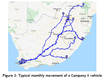
Analysing the collected data is undeniably one of the project's most challenging and important steps. Understanding how a vehicle travels, and relating this to the collected data from Step 3, is more complex than it might seem. The easiest method to analyse and understand the data is to illustrate a vehicle's movement visually, as shown in Figure 3. A visual representation of a vehicle's movement provides more insight into the route travelled, the delivery and collection locations, and points of interest such as depots, fuel stations, and wash bays. Figure 3 shows the movement of a single truck for a month, during which several trips across South Africa were made. From Figure 3, it is evident that the particular asset travelled mostly in and around Cape Town and between Cape Town and Pretoria. It also completed two trips to Durban, one to East London, and one to Limpopo. All of the other vehicles' trips were analysed similarly.

 

 

The visual representation of asset movements helped to identify the standard format of a 'trip'. This identification would have been overlooked if a visual analysis had not been performed. All trips follow the process shown in Figure 4, independent of the type of product in the tanker, customer, or delivery location. Starting at a depot, a fully fuelled truck with a clean tanker travels to the point of collection. Here the tanker is filled with cargo and then it travels to the delivery location. After offloading the cargo at the delivery location, the truck and empty trailer return to a depot to be washed and refuelled before the next trip starts. Washing the tanker after each load is essential, since the cargo is food products, and strict sanitary protocols are followed to avoid the contamination of food products.

 

 

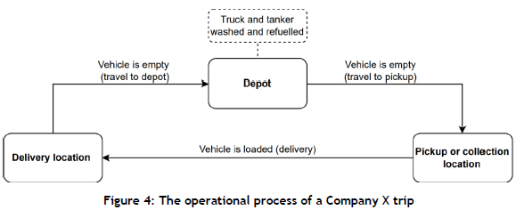
The only exception to the operational process described in Figure 4 was if the type of product allowed for repeat loads without washing the tanker. None of the analysed trips, however, fell into this exception category. The movement to and from a depot is typically empty, while the movements between other points of interest are loaded. For Company X, a 'new' trip begins when a vehicle visits a depot, its fuel tank is filled, and the tanker compartments are washed.

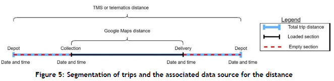
This identification of the operational process allowed the researchers to split each trip and its associated data into different segments, as shown in Figure 5. This trip segmentation is a prerequisite to performing the calculations in Section 3.5. From Figure 5, it can be seen that two different distances were used: the total trip distance from the TMS or the vehicle telematics system, and a Google Maps distance between the collection and delivery locations. The total trip distance was determined by aggregating the distance values between two timestamps (departure and arrival date and time) in the TMS and the vehicle telematics system. The maximum distance between the TMS and the vehicle telematics system was selected as the total trip distance. The Google Maps distance was calculated, assuming that trucks follow the shortest feasible road distance between the collection and delivery locations. Both distances validated each other, since the Google Maps distance should have been shorter than the total distance obtained from either the TMS or the vehicle telematics system.

A visual analysis also validated the timestamps, since the movement of a vehicle needed to correlate with these timestamps. In addition, geolocations indicated whether a vehicle was stationary or moving. This helped to identify and explain instances where a vehicle was parked at a depot or was waiting to be loaded or offloaded. Using geolocations and timestamps ensured that each trip was correctly divided in to loaded or empty sections, according to Figure 5. The equations stated in Section 3.5 were then applied to each trip to calculate an EIF for that trip.

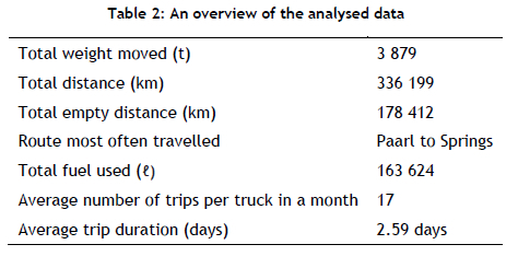
Since the EIF is calculated based on the loaded kilometres (tonne-km), segmenting trips into loaded and empty segments is vital. In addition, calculating the percentage of the empty running or 'lost' kilometres of a trip requires that trips be segmented accordingly. Using the described analysis process, 134 trips, of which six were milk runs, were analysed. A summary of the dataset is shown in Table 2, from which it is evident that a significant amount of cargo (3879 t) was transported by the eight vehicles in 134 trips. It is important to note that more than half of the total travel distance was empty. This could be ascribed to the dedicated equipment type used for bulk liquid transport that cannot be used for other purposes.

 

 

5. RESULTS

The results of the paper are discussed in three sections. The first section discusses the entire dataset, while Section 5.2 gives the results based on specific routes (N1, N2, N3, and N3-N5-N1). The third section, Section 5.3, assesses the results of specific origin-destination city pairs.

5.1. Entire dataset

Table 3 states the average EIF for the entire dataset, calculated according to the US EPA's SmartWay methodology [9]. The total tonne-kilometre value in Table 3 is the sum of each trip's tonne-kilometre value. From this tonne-kilometre value, it is evident that a significant amount of freight was shifted in the three-month analysis period. It is also notable that the 134 trips consumed over 163 k€ of diesel, resulting in about 507 t of CO2e emissions. The basis for results in Table 3 indicates the empty running and loading profile for the entire dataset. In total, 53.1% of all vehicle kilometres travelled were empty or 'lost' kilometres. In addition, if a vehicle was carrying a load, the truck was only loaded to 68.7% of its possible 36 t payload capacity. On average, if Company X moves a tonne of cargo a kilometre, 0.130 kg CO2e is emitted.

This value is 106% greater than the GLEC framework factors for Europe and South America, and 69% greater than the GLEC's proposed factor for Africa, which has a conservative load factor of 60% and an empty running value of 17%.

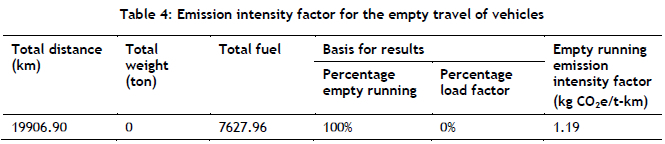
Analysing the data in Section 4 revealed that Company X's vehicles were often repositioned empty between trips to a different depot. The emissions from inter-depot repositioning cannot be allocated to trips carrying cargo, since this would penalise some customers while others would be advantaged. Thus an empty running EIF (kg CO2e/km) was also derived for Company X's fleet, as shown in Table 4. According to Table 4, an empty truck emits 1.19 kg CO2e per kilometre travelled. Note that the unit of the empty running EIF is only distance-based (km travelled).

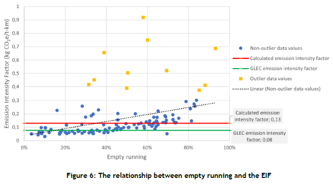
After the average EIF for both loaded and empty travel had been determined, all trips were assessed to identify how the empty running and the load factor of the vehicle affected the EIF. The EIF was plotted against each trip's empty running and load factor, as indicated in Figures 6 and 7. Note that the yellow square values in Figures 6 and 7 indicate outliers according to the 1.5 interquartile rule. These outlier values were omitted from Table 3's results or any other results in the paper, since they would have skewed the results disproportionally. These trips could be described as special cases with low load factors to avoid instances of completely empty repositioning.

Analysing the results in Figure 6 revealed a positive correlation between the EIF and the percentage of empty running, as shown by the trendline in Figure 6. This means that, as the proportion of distance travelled empty increases, the EIF also increases. The opposite is true for a vehicle's load factor and EIF, as indicated by the trendline in Figure 7. As the load factor increases, the EIF decreases, indicating a negative correlation. This means that the emissions from a trip do not increase in proportion to the vehicle load.

Apart from displaying the calculated EIF, Figures 6 and 7 also show the results compared with the proposed GLEC factors. The proposed GLEC EIF of 0.080 kg CO2e/t-km (horizontal green line) shows that a significant number of data values lie above the suggested factor. The same applies to the adjusted EIF (red horizontal line), which indicates the 22% that was added to account for the GLEC's proposed African operational conditions.

From Figures 6 and 7, it is evident that the number of trips assessed needs to be increased significantly to provide more reliable results. The EIFs in these two figures are far apart, and further analysis of additional trips should be used to determine whether these points are representative.

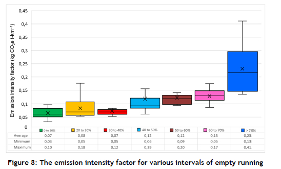
It is also clear from Figures 6 and 7 that the empty running of a vehicle has a more significant impact than the load factor of the vehicle. Subsequently, Figure 8 was developed to investigate the impact of different empty running intervals. Figure 8 shows a box-and-whisker plot for each interval of empty running and a data table indicating the average, minimum, and maximum EIFs in the range. Two important observations are made from Figure 8: as the empty running interval increases, so does the EIF; and the smaller interquartile range of the box-and-whisker diagram, the more consistent the results are.

 

 

5.2. Route-based

The second type of analysis is based on the intuition that the EIF is linked to the route travelled. Every route is different in respect of the elevation gain, the average traffic conditions or congestion, and the waiting or idle time at weighbridges and in urban areas. Thus the dataset of 134 trips was assessed to identify which trips travelled specifically on national roadways. Only national roadways needed assessment, since Section 4's analysis showed that Company X's vehicles prefer national roadways (N-routes) instead of secondary roadways (R-routes). The results of the route-based analysis are shown in Figure 9. Also, note the data table in the figure that states each route's average, minimum, and maximum EIF. Company X's vehicles predominantly travel four routes: the N1, the N2, the N3, and a combination of the N3-N5-N1 from Durban to Cape Town. The results in Figure 9 assessed bi-directional origin-destination trips on the routes, meaning that trips in both directions were assessed.

 

 

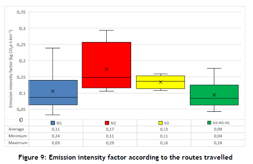
The box-and-whisker diagram in Figure 9 shows that each route has a sizeable interquartile range, except for the N3, which has a smaller variation. Despite the variation, it is clear that there is a difference in the average EIF between the different routes. All routes, however, require that more trips be accessed to increase confidence in the results.

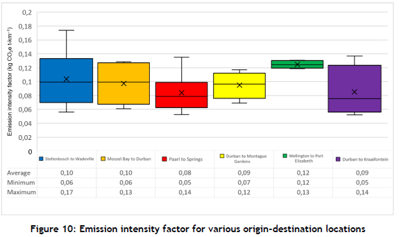
5.3. Origin-destination pairs

The origin-destination pairs analyse the trips of Company X's clients between specific cities. This differs from the route-based results, since the origin and destination locations are more refined, which intuitively would give more consistent results. From Figure 10, it is clear that there is still a significant variation in the EIF, even though the same origin-destination pairs were assessed. The exception is trips from Wellington to Port Elizabeth, which have more consistent results. All other origin-destination pairs require more assessment, since the range of results is quite large.

 

 

6. CONCLUSION

This paper established an EIF for a road-freight transporter, Company X, that transports bulk liquids in South Africa. The project assessed eight trucks' logistical activity and movement for three months, during which 134 trips were completed. The results revealed that, on average, if Company X moves a tonne of cargo a kilometre, 0.130 kg CO2e is emitted. This factor enables Company X to determine how much is emitted by a typical shipment, and allows for internal benchmarking to gauge progress in reducing emissions. Although not for tankers specifically, the EIF of 0.130 kg CO2e/t-km is 106% greater than the GLEC framework's factor for Europe and South America, and 69% greater than the GLEC's proposed factor for Africa, which has a similar load factor but a lower percentage of empty running. It is evident that the generic EIF in the GLEC framework significantly underestimates the emissions, and that more detailed EIFs should be stated in the GLEC framework or other literature sources.

The tanker industry is unique in the road-freight sector, since tankers must be cleaned after each trip. This is particularly relevant for Company X, since they transport food products, for which strict sanitary protocols apply. The cleaning requirement led to an empty running or 'lost' kilometres of 53.1%, meaning that more than half of the total distance travelled was unladen. If Company X wishes to reduce its emissions, the percentage of empty running must be reduced dramatically. However, this requires a financial investment either to create more depots at strategic locations or to outsource the cleaning of tankers to companies near the delivery or collection locations, which might not be financially feasible.

From the analysis, it was also evident that, in Company X's case, empty running has a larger impact on the EIF than the load factor. As a result, the impact of empty running on the EIF was assessed for various routes and origin-destination pairs. Although Sections 5.1 and 5.2 show the potential of a route and origin-destination assessment, a more extensive dataset is required to provide more consistent and trustworthy results. The authors advise Company X to use the EIF stated in Figure 8. If the empty running value is unknown, the average conservative EIF of 0.130 kg CO2e/t-km must be used.

This paper shows that the road-freight sector is very carbon-intensive. If South Africa wants to achieve its ambitious emission reduction goals, a radical transformation is required. Furthermore, decarbonising the road-freight sector would require substantial investments in driver training, newer vehicle technology, lower carbon fuels, aerodynamic fixtures, lightweight trailers, and similar aspects. Road-freight companies should also optimise their route planning to limit a vehicle's empty travel. A combination of investment and route optimisation is essential to increase the efficiency of transport activity, which would reduce emissions. With rising fuel prices, road-freight companies should come to understand the importance of streamlining business operations, potentially leading to a reduction in emissions. The potential of a modal shift to a less carbon-intensive mode such as rail transport should also not be ruled out. Although rail is not suitable for the type of commodity analysed in this paper, other bulk commodities such as coal and ore are ideal candidates for rail transport.

Significant future work is required in the road-freight industry - not only in terms of a standard emission estimation methodology, but also concerning the data collection and analysis process. Data collection is a big challenge if a company's departments function in 'silos', leading to challenges in identifying related trip data. Further, the analysis process is tedious; so it is hoped that organisations could collect data in the future during the business process or by identifying collective datasets related to trips. This would avoid a 'post- mortem' of multiple extensive datasets to understand the movement of vehicles and the associated data.

 

REFERENCES

[1] J. Bateh, C. Heaton, G.W. Arbogast, & A. Broadbent, "Defining sustainability in the business setting," Journal of Sustainable Management, vol. 1, no. 1, pp. 1-4, 2014.         [ Links ]

[2] C.I. Apetrei, G. Caniglia, H. von Wehrden, & D.J. Lang, "Just another buzzword? A systematic literature review of knowledge-related concepts in sustainability science," Global Environmental Change, vol. 68, no. 2021, 102222, 2021.         [ Links ]

[3] S. Schaltegger, & R. L. Burritt, "Corporate sustainability accounting: A nightmare or a dream coming true?" Business Strategy and the Environment, vol. 15, no. 5, pp. 293-295, 2006.         [ Links ]

[4] Z. Rezaee, & L.Tuo, "Are the quantity and quality of sustainability disclosures associated with the innate and discretionary earnings quality?" Journal of Business Ethics, vol. 155, no. 3, pp. 763-786, 2019.         [ Links ]

[5] A. Mckinnon, Decarbonising logistics: Distributing goods in a low-carbon world, 1^st ed., New York: Kogan Page, 2018.         [ Links ]

[6] M.J. du Plessis, J. van Eeden, & L. Goedhals-Gerber, "Carbon mapping frameworks for the distribution of fresh fruit: A systematic review," Global Food Security, vol. 32, no. December 2021, 100607, 2022.         [ Links ]

[7] S. Greene, and A. Lewis, Global logistics emissions council framework for logistics emissions accounting and reporting, Smart Freight Centre, 2019.         [ Links ]

[8] A.C. McKinnon, & M. Piecyk, Measuring and managing CO2 emissions of European chemical transport, Brussels: European Chemical Industry Council (CEFIC), 2012.         [ Links ]

[9] U.S. Environmental Protection Agency, 2021 SmartWay Logistics Company partner tool: Technical documentation, 2021.         [ Links ]

[10] IPCC Secretariat, The evidence is clear: The time for action is now. We can halve emissions by 2030, IPCC Working Group III, 4(April), 2022.         [ Links ]

[11] South Africa Department of National Treasury, Reducing greenhouse gas emissions: The carbon tax option, Discussion paper for public comment, 2010.         [ Links ]

[12] KPMG. "South Africa: Extension of carbon tax in budget 2022", 2022. [Online]. Available: https://home.kpmg/us/en/home/insights/2022/02/tnf-south-africa-extension-carbon-tax-budget-2022.html. [Accessed: 09-Jun-2022].         [ Links ]

[13] WBCSD & WRI, The greenhouse gas protocol: A corporate accounting and reporting standard, rev. ed., Geneva, Washington DC: WBSCD & WCI, 2004.         [ Links ]

[14] M. Coppola, & J. Blohmke, "Feeling the heat?: Companies are under pressure on climate change and need to do more," 2022. [Online]. Available: https://www2.deloitte.com/us/en/insights/topics/strategy/impact-and-opportunities-of-climate-change-on-business.html. [Accessed: 14-Jun-2022].         [ Links ]

[15] F. Ahjum, B. Merven, A. Stone, and T. Caetano, "Road transport vehicles in South Africa towards 2050: Factors influencing technology choice and implications for fuel supply," Journal of Energy in Southern Africa, vol. 29, no. 3, pp. 33-50, 2018.         [ Links ]

[16] Department of Transport, Republic of South Africa, Green transport strategy for South Africa: (2018-2050), Pretoria: Department of Transport, 2018.         [ Links ]

[17] F. Ahjum, C. Godinho, J. Burton, B. McCall, & A. Marquard, "A low-carbon transport future for South Africa: Technical, economic and policy considerations," Energy Systems Research Group, University of Cape Town, South Africa, March 2020.         [ Links ]

[18] H. Reid, "UPDATE 2 - South Africa's Transnet declares force majeure on coal contracts, Thungela says," 2022. [Online]. Available: https://www.reuters.com/article/safrica-mining-transnet-idUSL2N2WC0MR. [Accessed: 06-Jun-2022].         [ Links ]

[19] A.K. Kamdar, 2021. Road freight sustainability 4.0. Transport Action Group.         [ Links ]

[20] BSI & BS, "Methodology for calculation and declaration of energy consumption and GHG emissions of transport services (freight and passengers)," EN 16258:2012, 31 Dec., 2012.         [ Links ]

[21] WBCSD & WRI, Technical guidance for calculating Scope 3 emissions, World Resources Institute & World Business Council for Sustainable Development, 2013.         [ Links ]

 

 

* Corresponding author: martinduplessis6@gmail.com
ORCID® identifiers
M.J. du Plessis: 0000-0001-9668-3253
J. van Eeden: 0000-0001-9684-2357
M. Botha: 0000-0003-0009-8792