


Serviços Personalizados
Artigo
 Inglês (pdf)
 Artigo em XML
 Referências do artigo
Indicadores

Links relacionados
-
 Citado por Google
 -
 Similares em Google
Compartilhar

 Permalink
South African Journal of Industrial Engineering
versão On-line ISSN 2224-7890
versão impressa ISSN 1012-277X
S. Afr. J. Ind. Eng. vol.33 no.1 Pretoria Mai. 2022
http://dx.doi.org/10.7166/33-1-2553
GENERAL ARTICLES
Assessment of forecasting methods to reduce the margin of error in electronic component sales
A. MaldonadoI; R.D. LópezI, *; H. JassoI; G. HuertaI, II; J.A. RodríguezIII
ITecnológico Nacional de México/Campus Cd. Victoria, México. Department of Mechanical Engineering
IITecnológico Nacional de México/Campus Cd. Victoria, México. Division of Graduate Studies and Research
IIIUniversidad Politécnica de Victoria, México. Department of Engineering and Manufacturing
ABSTRACT
International competition in the electronic market requires that organisations use their resources not only to manufacture high quality components, but also to adopt or develop appropriate sales forecasting methods that could adapt to their needs and guarantee their economic development. From an industrial engineering perspective, keeping balanced orders and healthy safety stocks is required for such organisations. These two metrics play a significant role in their economic growth and development, because any disruption results in high costs throughout their manufacturing processes. Thus significant resources are spent by these organisations to develop information systems and logistics skills in order to implement more reliable and precise sales forecasting methods. Nevertheless, planners and forecasters constantly face different challenges such as sudden demand changes, seasonality, products with a short life cycle, a lack of historical data, and swings in the world economy. The objective of this research is to determine the most convenient demand forecasting method for the manufacturers of electronic devices that target a specific market. Twenty-seven months of sales data were analysed and different quantitative forecasting methods were tested and analysed using statistical tools. From the results obtained, the combined forecasting method appeared to be the most suitable since the least amount of forecasting error is obtained when this method is applied. The results of this research could be adopted by other companies to forecast the future sales of any items with a similar pattern to that used in our study. This has significant implications for their decision-making processes and inventory planning.
OPSOMMING
Internasionale mededinging in die elektroniese mark vereis dat organisasies hul hulpbronne nie net gebruik om komponente van hoë gehalte te vervaardig nie, maar ook om toepaslike metodes om verkope te voorspel aan te neem of te ontwikkel wat by hul behoeftes aanpas en ekonomiese ontwikkeling kan waarborg. Vanuit 'n bedryfsingenieurswese-perspektief is die hou van gebalanseerde bestellings en gesonde buffer voorraad vir sulke organisasies nodig. Hierdie twee maatstawwe speel 'n beduidende rol in hul ekonomiese groei en ontwikkeling, want enige ontwrigting lei tot hoë koste regdeur hul vervaardigingsprosesse. Beduidende hulpbronne word dus deur hierdie organisasies bestee om inligtingstelsels en logistieke vaardighede te ontwikkel ten einde meer betroubare en presiese verkope voorspellingsmetodes te implementeer. Nietemin staar beplanners en voorspellers voortdurend verskillende uitdagings in die gesig, soos skielike vraagveranderinge, seisoenaliteit, produkte met 'n kort lewensiklus, 'n gebrek aan historiese data en siklusse in die wêreldekonomie. Die doel van hierdie navorsing is om die mees gerieflike metode vir die voorspelling van vraag te bepaal vir die vervaardigers van elektroniese toestelle wat 'n spesifieke mark teiken. Sewe-en-twintig maande se verkopedata is ontleed en verskillende kwantitatiewe voorspellingsmetodes is met behulp van statistiese instrumente getoets en ontleed. Uit die resultate wat verkry is, het die gekombineerde voorspellingsmetode die geskikste geblyk te wees aangesien die kleinste voorspellingsfout verkry word wanneer hierdie metode toegepas word. Die resultate van hierdie navorsing kan deur ander maatskappye aangeneem word om die toekomstige verkope van enige items met 'n soortgelyke patroon as wat in ons studie gebruik is, te voorspel. Dit het beduidende implikasies vir hul besluitnemingsprosesse en voorraadbeplanning.
1 INTRODUCTION
Competitiveness in the electronic component markets has aroused the attention of business executives, especially on the flow of materials inside the supply chain. For most companies, the functionality of the supply chain is an area with high uncertainty, and even though the companies invest resources in improving their forecast sales methods, constant changes in the economy of international markets require actions to adjust their forecasts and decrease their error margins. Organisations competing worldwide in the electronic market are focused not only on the development and manufacturing of high-quality electronic devices, but also on the implementation of sales forecasting methods that consider the multiple variables influencing international trade. Therefore, companies focus much of their effort on developing information systems and logistics skills that allow them to develop more accurate and more reliable sales forecasts [1]. However, day-to-day planners and forecasters deal with multiple limitations in international markets, such as sudden changes in demand levels, seasonality, products with short life periods, a lack of historical data, and large swings in the world economy.
In recent years, various sales forecasting techniques have been applied in studies [2]. These techniques have contributed to the development of a more assertive decision-making process by reducing the margin of error caused by the high variability and complexity in international markets. The success of a forecast lies in selecting the technique that best matches the characteristics and variables of the product market under analysis. Both the manager and the forecaster play a very important role in the organisation and the better they understand the possibilities and alternative solutions, the closer they will be to forecasting with greater chances of success. A significant number of companies worldwide (specifically in the manufacturing industry) require a reliable sales forecast, since they are unable to know precisely the future demands of their products. Thus they have to rely on demand forecasts to plan their long-term business strategies and to ensure that the supply chain operates effectively. As a result, these companies have adopted different demand forecasting methods based on both their sales history and the situation of international markets [3]. Therefore, the ability to make demand forecasts with a high level of accuracy plays an important role in today's organisations.
Supply chain management, if carried out properly, generates added value to the operations of the manufacturing process, helping to maintain profitability in business operations. Therefore, improving demand forecasting performance has been the main concern of many manufacturing companies for many years, and remains so [4-6].
The complexity of making a good forecast has led to the development of new forecasting techniques and methods in the last three decades. They are essential for planners, forecasters, and company managers to make accurate predictions and decisions about the demand for their products in the short, medium, and long term. It is important to note that each forecasting method has different advantages and disadvantages. Here the forecasters and planners of each company play a significant role in the choice of the forecasting method, which is associated with the internal factors related to the product and the economic situation of the world market. Among them is the context of the forecast, the relevance and quantity of historical data, the desired degree of precision, the period to be forecast, the cost-benefit relationship, the time available to carry out the study, and its costs, scope, and accuracy.
Knowledge of market conditions improves sales forecasts. Most forecasts, regardless of the method selected, are not 100 per cent accurate, leaving opportunities for error. Some researchers have decided to combine qualitative and quantitative methods for demand forecasting, obtaining favourable results and so reducing the margin of error [7-8].
This research was developed in a company with more than twenty years in the electronic products market. The case study focused on the forecast of sales of electronic capacitors. Traditionally this company has used the simple moving average (SMA) method for its sales forecasts, maintaining an error above 15 per cent for the European market according to its historical sales data, which means a significant economic loss. The objective of this research was to determine a sales forecast method that guarantees an error margin below 10 per cent. To achieve this objective, the historical sales data was analysed and a forecasting method was proposed that was based on the least difference between the real sales data and the projection. The quantitative sales forecast methods that were analysed were simple moving average, linear regression, and seasonality combined with linear regression.
2 LITERATURE REVIEW
Different forecasting techniques can be applied in organisations depending on their business activities. These techniques are divided into two categories: qualitative and quantitative. The qualitative approach tends to predict the future when no historical data is reliable or available to forecast demand products. This approach is based on the judgements and opinions of management, forecasters and/or planners with extensive experience in their companies. The quantitative approach is divided into time series methods (forecasts based on historical data) and explanatory methods (application of regression, exponential smoothing, models of AutoRegressive Integrated Moving Average (ARIMA), and others) [9]. This approach can also consider econometric models and global economic indicators.
2.1 Qualitative forecasting methods
When making important decisions, qualitative methods still hold high importance for managers and forecasters. Qualitative methods are not limited to the industrial or project organisation fields; they can be applied to social and economic development too, such as the growth of a country [9]. For many years, a significant number of works has been developed using this method, with very favorable results for the growth of organisations [10-14]. Some researchers [15-17] have used integrated methodologies such as judgemental adjustment, the 50-50 combination, divide-and-conquer, and the consensus forecasting method, and have highlighted the importance of having experienced forecasters in their companies to make adjustments when the prediction from their results is very high. On the other hand, the need to consider various methods of qualitative analysis is emphasised owing to the high level of competition in national and international markets, which highlights the absence of information in time series [18].
Although the analytical methods used in this investigation were based on quantitative forecasting methods, qualitative methods especially the consensus method were applied as part of the company forecasters' decision-making process. These methods are usually applied by individuals or committees in a consensus process to reach an agreement, and to make decisions when there is some level of uncertainty. The application of consensus forecasts is based on a method that considers the analysis and interpretation of data over time and on different levels of analysis that are agreed upon from an organisational perspective. Each part of the organisation that is involved makes its individual forecast, and then a team meeting is held and consensus is reached. Most research using consensus methods among forecasters has focused on the evaluation of quantitative forecasts [19-20]. Although most of these investigations have used time series data to make their forecasts, more recent studies have suggested the application of dispersion, simple moving averages, and distribution analysis for this type of forecast [21-22]. Prior research on the accuracy and efficiency of the consensus forecast showed that forecasters use historical data and current market situations to predict demand or to forecast their sales. If these predictions are efficient, they will provide correct and timely information so that forecasters have the necessary and relevant information for their decision-making.
2.2 Quantitative forecasting methods
Sales forecasting is an integral part of any company. Therefore, any manager or executive should consider the importance of selecting an adequate forecasting method for a specific situation, in which they consider the strengths and weaknesses of each approach. A wide range of different approaches and methods is used nowadays in forecasting practice. Quantitative methods generally focus on statistical mathematical techniques, numerical calculations, the use of simulation software to predict future events [23] and using trend analysis and trend extrapolation. Researchers [24-26] use a combined forecast analysis that considers different analysis methods. In this research, different quantitative forecasting methods have been used to obtain a sales projection with the minimum dispersion under the company's sales conditions. The advantage is that multiple combinations of forecasts can be made, thus taking full advantage of each forecast without the calculation of the combined method becoming complex.
A significant number of forecasting methods is available in the literature, such as simple moving average, linear regression, weighted moving average, linear regression and seasonality, and exponential smoothing.
These methods have demonstrated their efficiency not only in predicting sales forecasts, but also in many other areas of knowledge.
Linear regression is a technique used to estimate the behaviour of a series of data and to determine whether two or more variables are related. Several mathematical equations are part of this technique. The purpose of a linear regression equation is to estimate the value of an unknown variable, based on the known values of others. Although linear regression can take various forms for its interpretation and analysis, the simple linear regression model is of great interest for the present investigation because of its simplicity and accuracy. Typically, linear regression is used in long-term forecasts.
Studies conducted by Ade-Ikuesan et al. [27], Ciulla and D'Amico [28], and Jonsson [29] have used the linear regression method to improve the behaviour of different events such as adjusting market predictions, improving consumption trends, and decreasing the percentage of error by estimating and improving sales forecasts in unpredictable markets.
The simple moving averages method is a short-term time series forecast model. Its main objective in the sales context is to forecast sales for the next sales period. When the sales forecast is calculated using the simple moving average method, mathematical analysis is used to calculate the average sales value over the next given period of time using a fixed number of historical data. When the calculated average value is higher than the real value, we say that the number is overestimated. On the other hand, if the average value is lower than the real one, we say that the number of sales is underestimated. In both cases, action must be taken to adjust the forecast. In a cumulative average, each value of the new series is equal to the sum of all previous values. This technique is used to measure the variation in the sale of a product or the number of sold pieces. Two or more data can be averaged to obtain the prediction value. Recent research has used the moving averages method to improve the accuracy of sales forecasts in different markets. The results of this method have shown an increase in profit margins and improved systems [30-31]. Whereas it is true that forecasting using the moving averages method is simple, forecasters often use it as an information base for more complex time series forecasting methods.
2.3 Combined forecasting methods
Combined forecasting methods were developed 50 years ago [32]. Since then, different forecasting combinations have been adopted and implemented, resulting in a greater number of available options for managers and forecasters to select a forecast method or model that fits their commercial needs [33]. To determine which method and forecast model should be applied in a specific case, several forecasting methods should be evaluated to eliminate unsuitable models, even if they tend to improve performance [34]. The effectiveness of forecasting methods used to predict demand depends on different factors, such as the time available to forecasting, trend and seasonality patterns existence, and the behaviour of the demand for an estimated time. The evaluation of these factors depends on the forecast's acceptable level of error and its effectiveness. When forecasting methods are combined, the margin of error can be reduced. Several researchers [35] have shown that combined forecasts generally exceed the prognosis of the best individual model. The present investigation considered a combined forecasting method using linear regression forecasts with seasonality.
The sales forecast of electronic components is a complex prediction problem that includes multiple variables such as seasonality, changes in the market, and product lifetime. Since these variables are not constant over time, it is not an easy task to determine their importance level. However, having a method of sales forecasting helps companies to reduce the margin of error associated with predictions. Measuring forecast errors improves forecast accuracy: the smaller the forecast error, the more accurate the method [36].
3 RESEARCH DESIGN
The objective of this study was to determine the most suitable sales forecasting method - one that would guarantee an error margin of below 10 per cent - for a company that manufactures electronic components and whose primary customers are in the European market. Including individual and combined sales forecasting methods, different methods were used to achieve the expected objective. It is relevant to point out that not all the tested methods are reported in this work; so the next section only shows the sales forecasting methods with the highest probability of success for the market that was analysed.
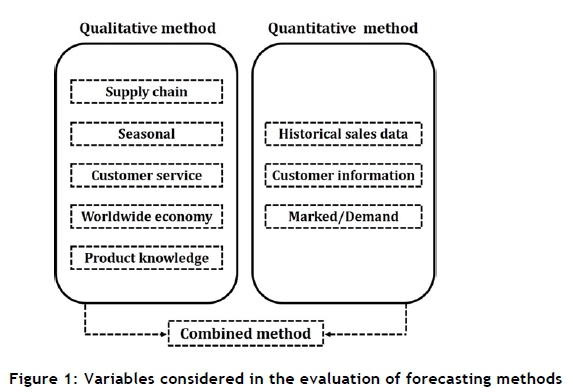
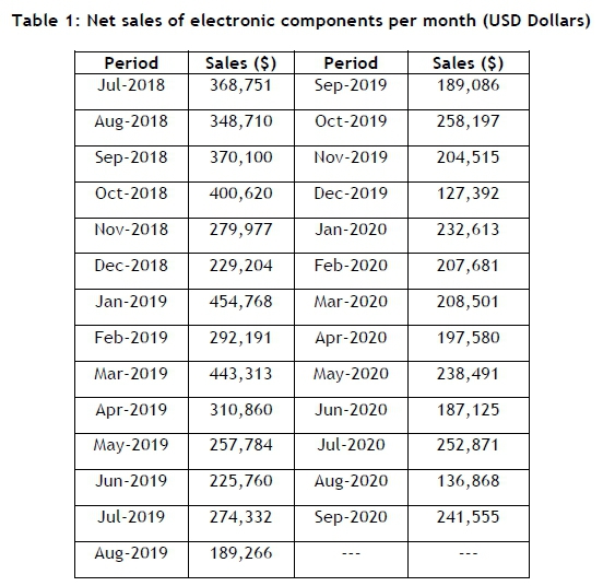
Figure 1 shows the variables that were studied as part of the qualitative and quantitative methods. Only some of these variables (historical sales data, market/demand, seasonal, and supply chain) were evaluated in this work. The sales data of electronic components from 27 consecutive months were analysed, as can be seen Table 1. Although the company manufactures more than 80 types of electronic component, and has a presence on five continents, the analysis of the research focused on the product with the greatest demand in the European market.
3.1 Simple linear regression analysis
Data analysis using simple linear regression is a widely used statistical tool. The tool tries to explain the relationship between a response variable Y and a single explanatory variable X. The objective of the linear regression technique is to find an equation that represents the relationship between both variables (X¡, Yt) with the least possible error. The linear regression equation is presented in equation (1):

The linear regression equation with the least possible error is found solving equation (2):

where Y¡ is the solution of the equation for the value X¡. ß0, and ßlare the model parameters (regression coefficients), the coefficient ß0called constant is the expected value of Ywhen X=0, and the coefficient ßj, called the slope, is the change in Yinfluenced by the amount of change in X Xiis the predictor and είis an error term. Given a set of points Xand Y, the solution will be given by equation (3):
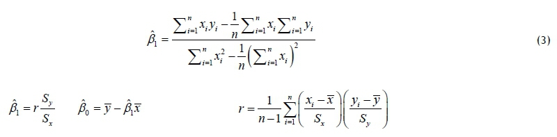
where  ,
, , Sxand Syare the sample averages and standard deviations for the values of x and y respectively, and r is the correlation coefficient.
Because it is a relatively easy forecasting method to be simulated when sufficient historical sales data is available, the simple linear regression method was selected as a sales forecasting model for this research. The data, when manipulated, generate a dispersion system; when running the corresponding simulation method, its linear regression is obtained, which provides information about the degree of variation represented by the data. Linear regression is also the method that has been used by the company where this study was developed.
3.2 Simple moving averages
The objective of the simple moving averages technique is to make projections based on historical periods greater than 1. An arithmetic moving average is calculated by adding recent values and then dividing the result of this value by the number of time periods that are considered. Using several time periods can minimise the fluctuations that occur when using only a few periods. For example, in cases in which the historical periods are measured in months and a forecast is estimated using three-month moving averages for many particular months, the value obtained represents the average of each of those three months. The simple moving average (SMA) can be defined by the equation (4):
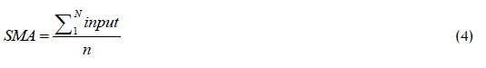
where n is the number of periods for which the SMA is numbered. The SMA smoothes the data, thus reducing noise and helping to identify trends. The SMA is the simplest form of a moving average. Each output value is the average of the previous n values. In an SMA, each value within the time period carries an equal weight to make it less sensitive to recent data changes. Values outside the time period are not included in the average.
Because the results obtained when applying the SMA method were closer to what was expected, this method was considered in the research. Although there were other forecasting methods, such as exponential smoothing, weighted moving averages, and trend and season (also simulated), the predicted average and standard deviation from the absolute error were far from acceptable. Therefore, they were not suitable for this case of sales forecasts for electronic components.
3.3 Linear regression and seasonality
Both techniques - linear regression and seasonality - can be combined to develop predictions based on historical data. If there is any season effect in the data, the seasonality analysis identifies, measures, and incorporates that effect into the forecast model. The first step is to calculate the average for each season. In the case of this study, it was decided to use four seasons (Q1, Q2, Q3, and Q4), each encompassing three periods - that is, three months - that corresponded with the company's financial reports for sales. The seasonal average was obtained using equation (5):
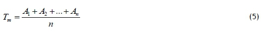
where T is the average of season m, A is the value of period n, n is the number of periods in the season, and m is the season number. Then a season index was calculated with equation (6):
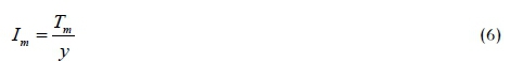
where y is the average of all actual output values.
Finally, a projection for each period/month was calculated by multiplying the value estimated through the linear regression for the selected period/month and the season index to which the period/month belongs, as can be seen in equation (7):
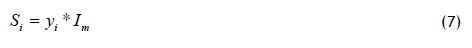
where S¡ is the projection of period I, ytis the projection of the linear regression, and Imis the season index to which y¡ belongs.
4 RESULTS
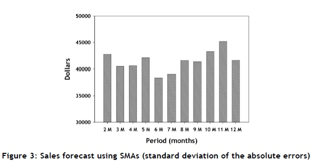
Figures 2 and 3 show the data for the SMA method. Because the most critical aspect of this method is to select the historical periods to be used, a range from two to 12 months was evaluated and compared. The mean absolute deviation (MAD) and the standard deviation of the absolute errors were calculated for each period.
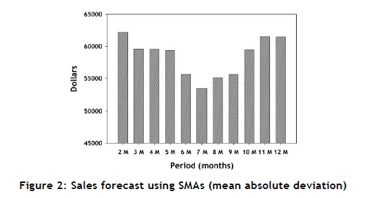
Figure 2 shows the MAD for the range selected. For each period tested, MAD was calculated using the average of errors for each month. Therefore, MAD gave an idea of how much the forecast value differed from the actual value in the evaluated months. According to the results, when a historical period of seven months was used, the least average error was obtained for those months (USD 53,575). Furthermore, when the sales forecast considered less than six months or more than nine months, there was an increase of 16 per cent on the average error, resulting in a negative financial impact. From a practical point of view, these findings could be relevant. Most companies face very competitive markets and keeping costs under control is vital. Figure 3 represents the standard deviation of the absolute errors for each period. When time periods from six to seven months were used to do the forecast, there was less dispersion than when shorter or longer periods were applied. The above is in accordance with what is used in this type of technique, in which it is suggested that an average of 200 days be used to obtain a lower margin of error.
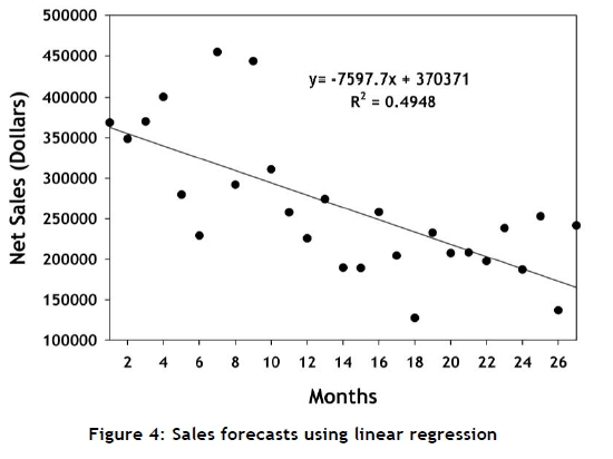
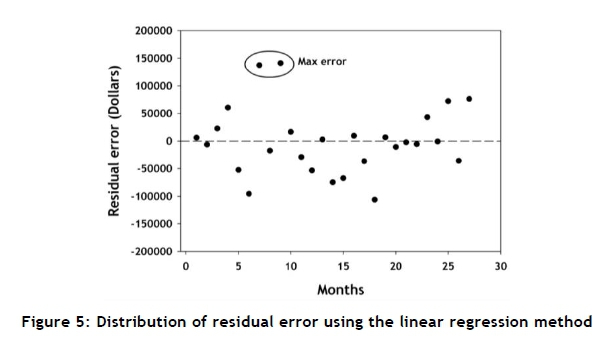
The linear regression analysis presented in Figure 4 was obtained from the sales data for electronic components for a period of 27 consecutive months, starting in July 2018. The straight line that appears in the figure represents the best fit for the data, and the difference between each point and the line is the residual error. The projected forecast shows a declining trend for sales. Even though there are months with acceptable predictions, there are others with significant errors. The distribution of the residual errors is plotted to validate the randomness of the sales data (Figure 5). It can be seen that the sales data per month do not show a clear trend, because they are far above and far below the line of control. Using this method, Nthe MAD is USD 44,063.
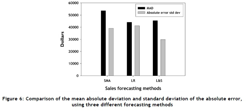
The sales forecast using the linearity and seasonality method is presented in Table 2. It is important to study both the seasonal fluctuations that might occur and the trends that might exist. Both can help to produce better sales forecasts. For this method, four seasons (Q1, Q2, Q3, and Q4) were used, each one covering three months per year. The average season was calculated using all the real values from the months belonging to that season, regardless of the year. After this, the seasonality index was calculated by dividing the previous average season by the average of all the months. The final forecast was the result of multiplying the value that was estimated by the linear regression by the seasonality index. From the results thus obtained, it can be seen that the mean absolute deviation (MAD) was USD 45,411, whereas the standard deviation of the absolute error was USD 29,837.
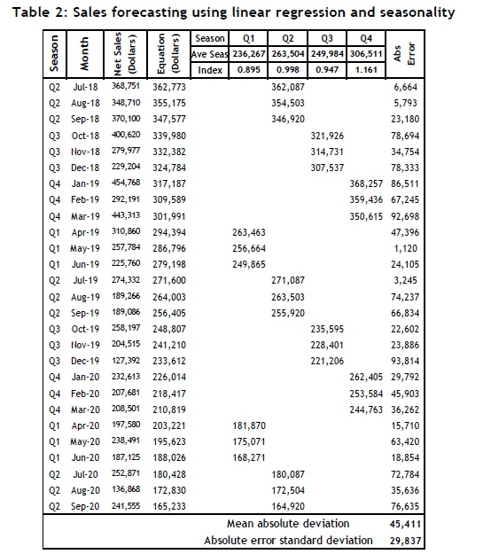
Figure 6 summarises the results of the three different forecasting methods in respect of the MAD and the standard deviation of the absolute error. The combined method using linear regression and seasonality (L&S) presented the best balance for MAD and the smallest standard deviation of absolute error. A comparison with the lowest MAD from the SMA method showed an improvement of 15.2 per cent when L&S was used. The simple linear regression (LR) method had the highest standard deviation of the absolute errors, which was higher than the value from the L&S.
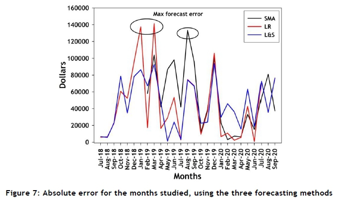
The absolute error for each month and each method is shown in Figure 7; the SMA and the linear regression method (SMA and LR) present the time periods with the highest errors, whereas the combined methods (L&S - blue line) show the smallest error, which match the results in Figure 6.
5 DISCUSSION
In recent decades a significant number of sales forecasting methods has been developed that consider the type of demand (secular trend, seasonal, cyclical, or irregular) or the time (short, medium, and long-term). Currently, forecasting with 100 per cent reliability is one of the most critical challenges for companies, regardless of industry and size. The error margins obtained from different forecasting methods showed that there is an appropriate forecasting method for the company's business conditions relating to the sales of electronic capacitors in the European market. Although all the studied methods showed errors in sales forecasting, SMA and linear regression showed a greater margin of error, unlike the combined method's error, which was within the company's acceptable limits.
It is critical to point out that, before this investigation, the company's forecasters and planners performed their predictions on the basis of only their experience. Even though a convenient database was available to help them to analyse sales trends, a lack of knowledge of forecasting methods limited its effectiveness, producing forecast errors above 15 per cent and incurring significant economic losses for the company.
Owing to multiple variables in the market and the supply chain, the sales forecast of capacitors is a challenging task to be considered. The company analysed in this research considers inventory levels, fluctuations along the supply chain, new product introductions, and the cost of materials - among others - to be critical and complex variables. For each forecasting method that was analysed, the error margin and objectives of the company were considered. Although applying forecasting methods might seem like a simple task, selecting the forecasting method that best suits a company's conditions is a challenge with far-reaching implications for its business.
Providing the company's forecasters with reliable tools to facilitate the decision-making process was one of the most important achievements of this project. These tools bring greater precision to the market demands and represent growth in the company's business. Using a single forecasting method - regardless of the changing situation worldwide - puts the company's interests at risk, since the demand for this type of product is not constant but fluctuates owing to various factors, such as those mentioned before. In the case of inventory levels, fluctuations are mainly because of the material stocked by the distribution companies, which might keep a considerable number of capacitors in their inventory, thus affecting the distribution channels. The proper functioning of a supply chain is achieved when it is effective and efficient. In other words, optimise your resources (human, financial, technological, and physical) in order to reduce both operating costs and wasted time, and to adapt to constant changes in the world economy. The fluctuating cost of raw materials is usually related to the internal situation in some producing countries, which may affect the markets for political and economic reasons. This situation is especially critical when a few countries control the sale of a specific material; with tantalum capacitors, for instance, only a few countries supply the demand for tantalum material.
6 CONCLUSION
Simple moving average, linear regression, and the combination of linear regression and seasonality were the methods evaluated to determine the best sales forecasting for electronic components, applying the margin of error as the main selection criterion. The historical data available in the company's database was used to undertake this evaluation.
Through the analysis of sales forecasting methods, several objectives were achieved, such as providing the company's forecasters with sufficient and reliable statistical tools for the decision-making process, improving the accuracy of their forecasts, decreasing their margin of error, and having a positive impact on the supply chain and the company's planning systems.
As shown earlier, the combined method (linear regression and seasonality) delivered the best results in respect of MAD and the least absolute error of the standard deviation, based on the current sales conditions of the company. The smallest errors could be transformed into improvements that would have a positive impact on sales forecasts, production costs, and profit margins.
The use of the combined forecasting method provides a better estimation of future sales. Performance metrics such as the inventory level, the stock of raw materials, the quantity of finished products, and others benefit from it, maintaining as little variation as possible on these metrics.
The results have shown the effectiveness of the combined forecast method when compared with the other methods that were studied. This has highlighted that the combined linear regression and seasonality method can forecast the sales of electronic capacitors for the European market with a reduction in the forecast error margin of less than 8.9 per cent, achieving the study's objectives. Therefore, it can be regarded as being acceptable. The combined method has the potential to be applied to predict the sales of the company's other types of electronic component and for different international markets.
The limitations of the selected method are focused on how to incorporate the experience and the qualitative information that the company studied here continues to use as input variables for decision-making. For instance, the experience and knowledge of the company's sales force provide valuable information that should, in the future, be incorporated in some way into the quantitative method. Currently this is performed in an unregulated way, with neither a method nor a procedure. This condition is a topic to explore in the future.
7 REFERENCES
[1] Fildes, R. & Hastings, R. 1994. The organization and improvement of market forecasting. Journal of the Operational Research Society, 45(1), pp 1-16. [ Links ]
[2] Davis, D. F. & Mentzer, J. F. 2007. Organizational factors in sales forecasting management. International Journal of Forecasting, 23(3), pp 475-495. [ Links ]
[3] Zotteri, G. & Kalchschmidt, M. 2007. Forecasting practices: Empirical evidence and a framework for research. International Journal of Production Economics, 108(1-2), pp 84-99. [ Links ]
[4] Siriram, R. 2016. Improving forecasts for better decision-making. South African Journal of Industrial Engineering, 27(1), pp 47-60. [ Links ]
[5] De Treville, S., Shapiro, R. D. & Hameri, A. P. 2004. From supply chain to demand chain: The role of lead time reduction in improving demand chain performance. Journal of Operations Management, 21(6), pp 613-627. [ Links ]
[6] Žic, J. & Žic, S. 2020. Multi-criteria decision making in supply chain management based on inventory levels, environmental impact and costs. Advances in Production Engineering and Management, 15(2), pp 151-163. [ Links ]
[7] Sanders, N. R. & Ritzman, L. P. 2004. Integrating judgmental and quantitative forecasts: Methodologies for pooling marketing and operations information. International Journal of Operations and Production Management, 24(5), pp 514-529. [ Links ]
[8] Franses, P. H. & Legerstee, R. 2009. Properties of expert adjustments on model-based SKU-level forecasts. International Journal of Forecasting, 25(1), pp 35-47. [ Links ]
[9] Stekler, H. & Symington, H. 2016. Evaluating qualitative forecasts: The FOMC minutes, 2006-2010. International Journal of Forecasting, 32(2), pp 559-570. [ Links ]
[10] Morikawa, M. 2019. Uncertainty over production forecasts: An empirical analysis using monthly quantitative survey data. Journal of Macroeconomics, 60(1), pp 163-179. [ Links ]
[11] Sanders, N. R. & Manrodt, K. B. 2003. The efficacy of using judgmental versus quantitative forecasting methods in practice. OMEGA International Journal of Management Science, 31(6), pp 511-522. [ Links ]
[12] Clements, M. P. 2008. Consensus and uncertainty: Using forecast probabilities of output declines. International Journal of Forecasting, 24(1), pp 76-86. [ Links ]
[13] Hassen, O. A., Darwish, S. M., Abu, N. A. & Abidin, Z. Z. 2020. Application of cloud model in qualitative forecasting for stock market trends. Entropy, 22(9), pp 991-1010. [ Links ]
[14] Doubravsky, K. & Dohnal, M. 2018. Qualitative equationless macroeconomic models as generators of all possible forecasts based on three trend values: Increasing, constant, decreasing. Structural Change and Economic Dynamics, 45 (C), pp 30-36. [ Links ]
[15] Alvarado, J. A., Barrero, L. H., Onkal, D. & Dennerlein, J. T. 2016. Expertise, credibility of system forecasts and integration methods in judgmental demand forecasting. International Journal of Forecasting, 33(1), pp 298-313. [ Links ]
[16] Arvan, M., Fahimnia, B., Reisi, M. & Siemsen, E. 2019. Integrating human judgement into quantitative forecasting methods: A review. OMEGA The International Journal of Management Science, 86(1), pp 237-252. [ Links ]
[17] Clarke, D. D. 1992. Qualitative judgemental forecasting methods for use in strategic decision making. International Conference on Information-Decision-Action Systems in Complex Organisations, Oxford, UK, pp 75-79. [ Links ]
[18] Naik, G. 2004. The structural qualitative method: A promising forecasting tool for developing country markets. International Journal of Forecasting, 20(3), pp 475-485. [ Links ]
[19] Ager, P., Kappler, M. & Osterloh, S. 2009. The accuracy and efficiency of the consensus forecasts: A further application and extension of the pooled approach. International Journal of Forecasting, 25(1), pp 167-181. [ Links ]
[20] Gregory, A. W., Smith, G. W. & Yetman, J. 2001. Testing for forecast consensus. Journal of Business and Economic Statistics, 19(1), pp 34-43. [ Links ]
[21] Byun, S. J. 2016. The usefulness of cross-sectional dispersion for forecasting aggregate stock price volatility. Journal of Empirical Finance, 36(C), pp 162-180. [ Links ]
[22] Lucas, A. & Zhang, X. 2016. Score-driven exponentially weighted moving averages and value-at-risk forecasting. International Journal of Forecasting, 32(2), pp 293-302. [ Links ]
[23] Esmaelian, M., Tavana, M., Di Caprio, D. & Ansari, R. 2017. A multiple correspondence analysis model for evaluating technology foresight methods. Technological Forecasting and Social Change, 125(c), pp 188-205. [ Links ]
[24] Terui, N. & Van Dijk, H. K. 2002. Combined forecasts from linear and nonlinear time series models. International Journal of Forecasting, 18(3), pp 421-438. [ Links ]
[25] Dekker, M., Van Donselaar, K. & Ouwehand, P. 2004. How to use aggregation and combined forecasting to improve seasonal demand forecasts. International Journal of Production Economics, 90(2), pp 151-167. [ Links ]
[26] Ivanyuk, V. 2018. Econometric forecasting models based on forecast combination methods. 11th International Conference "Management of large-scale system development", Moscow, Russia, pp 1-4. [ Links ]
[27] Ade-Ikuesan, O. O., Oyedeji, A. O. & Osifeko, M. O. 2019. Linear regression long-term energy demand forecast modelling in Ogun State Nigeria. Journal of Applied Sciences and Environmental Management, 23(4), pp 753-757. [ Links ]
[28] Ciulla, G. & D'Amico, A. 2019. Building energy performance forecasting: A multiple linear regression approach. Applied Energy, 253(1), pp 1-16. [ Links ]
[29] Jonsson, B. 1994. Prediction with a linear regression model and errors in a regressor. International Journal of Forecasting, 10(4), pp 549-555. [ Links ]
[30] Kolkova, A. 2018. Indicators of technical analysis on the basis of moving averages as prognostic methods in the food industry. Journal of Competitiveness, 10(4), pp 102-119. [ Links ]
[31] Lucas, A. & Zhang, X. 2016. Score-driven exponentially weighted moving averages and value-at-risk forecasting. International Journal of Forecasting, 32(2), pp 293-302. [ Links ]
[32] Bates, J. M. & Granger, W. J. 1969. The combination of forecasts. Operational Research Society, 20(4), pp 451-468. [ Links ]
[33] De Menezes, L. M., Bunn, D. & Taylor, J. W. 1999. Review of guidelines for the use of combined forecasts. European Journal of Operational Research, 120(1), pp 190-204. [ Links ]
[34] Timmermann, A. 2006. Forecast combinations. In Handbook of economic forecasting, San Diego, CA: North- Holland. [ Links ]
[35] Jiang, P., Liu, Z., Niu, X. & Zhang, L. 2021. A combined forecasting system based on statistical method, artificial neural networks, and deep learning methods for short-term wind speed forecasting. Energy, 217(1), p 119-361. [ Links ]
[36] Mentzer, J. T. & Moon, M. A. 2005. Sales forecasting management: A demand management approach. London: Sage Publications. [ Links ]
Submitted by authors 14 Jul 2021
Accepted for publication 26 Mar 2022
Available online 06 May 2022
ORCID® identifiers
A. Maldonado https://orcid.org/0000-0003-3585-8034
R.D. López https://orcid.org/0000-0002-2662-6103
H. Jasso https://orcid.org/0000-0003-4565-190X
G. Huerta https://orcid.org/0000-0003-0863-8159
J.A. Rodríguez https://orcid.org/0000-0002-6226-4242
* Corresponding author ricardo.lg@cdvictoria.tecnm.mx

