GENERAL ARTICLES

 

A variable sample size synthetic chart for the coefficient of variation

 

 

M. Yahaya^I; S.L. Lim^{I, *}; A.I.N. Ibrahim^I; W.C. Yeong^II; M.B.C. Khoo^III

^IInstitute of Mathematical Sciences, Faculty of Science, Universiti Malaya, 50603 Kuala Lumpur, Malaysia
^IIDepartment of Operations and Management Information Systems, Faculty of Business and Accountancy, Universiti Malaya, 50603 Kuala Lumpur, Malaysia
^IIISchool of Mathematical Sciences, Universiti Sains Malaysia, 11800, Penang, Malaysia

 

 

---

ABSTRACT

A variable sample size (VSS) synthetic chart to monitor the coefficient of variation (γ) is proposed in this paper to improve the performance of the existing synthetic χchart. A description of how the chart operates, as well as the formulae for various performance measures (i.e., the average run length (ARL), standard deviation of the run length (SDRL), average sample size (ASS), and expected average run length (EARL)) are proposed. The algorithms that optimise the out-of-control ARL (ARL1) and EARL (EARL1), subject to the constraints in the in-control ARL (ARL0) and ASS (ASS0), are also proposed. Subsequently, optimal charting parameters for various numerical examples are obtained. The proposed chart shows a significant improvement over the existing synthetic γ-chart. Comparisons with other γ-charts also show that the proposed chart performs better than the Shewhart- γand VSS-γcharts under all cases, while showing better performance than the exponentially weighted moving average (EWMA) and VSS EWMA- γ²charts for moderate and large shift sizes. Finally, this paper shows the implementation of the proposed chart on an actual industrial example.

---

OPSOMMING

'n Veranderlike Steekproefgrootte sintetiese grafiek om die variasiekoëffisiënt ( γ) te monitor, word in hierdie artikel voorgestel om die werkverrigting van die bestaande sintetiese grafiek te verbeter. 'n Beskrywing van hoe die grafiek werk, sowel as die formules vir verskeie prestasiemaatstawwe (d.w.s. die gemiddelde lopielengte, standaardafwyking van die lopielengte, gemiddelde steekproefgrootte en verwagte gemiddelde lopielengte) word voorgestel. Die algoritmes wat die buite-beheer gemiddelde lopielengte) en verwagte gemiddelde lopielengte optimeer, onderhewig aan die beperkings in die in-beheer gemiddelde lopielengte en gemiddelde steekproefgrootte, word ook voorgestel. Vervolgens word optimale parameters vir verskeie numeriese voorbeelde verkry. Die voorgestelde grafiek toon 'n aansienlike verbetering teenoor die bestaande sintetiese γgrafiek. Vergelykings met ander χ-grafieke toon ook dat die voorgestelde grafiek beter presteer as die Shewhart- χen Veranderlike Steekproefgrootte- γ²kaarte onder alle gevalle, terwyl dit beter prestasie toon as die eksponensieel geweegde bewegende gemiddelde γ²kaarte vir matige en groot skofgroottes. Ten slotte, hierdie artikel toon die implementering van die voorgestelde grafiek op 'n werklike voorbeeld in die industrie.

---

 

 

1 INTRODUCTION

By convention, most control charts monitor changes in the mean (μ) and/or standard deviation (σ) - for example, Coelho, Chakraborti and Graham [1], Teoh, Fun, Khoo and Yeong [2], and many others. However, not all processes have a constant μ. In addition, σmay change according to μ. One of the reasons this may happen is changes in process outputs as a result of different planning decisions, or it may be due to the inherent properties of the process. Dubious conclusions will be reached if such processes are monitored through conventional and R or S charts, since shifts in μand/or σdo not mean that the process is out of control (OOC).

A chart monitoring the coefficient of variation (γ) was first proposed by Kang, Lee, Seong and Hawkins [3], where For this type of chart, an OOC condition is only signalled with a change in the relationship between σand μ. In other words, as long as does not shift from the in-control (IC) value of γ, the process is IC. Yeong, Khoo, Tham, Teoh and Rahim [4] have reviewed several areas of application when monitoring γis important.

Numerous new charts are proposed to monitor γ, one of which is the synthetic chart by Calzada and Scariano [5]. The synthetic chart produces an OOC signal if successive samples falling outside the control limits are close to each other. It is preferred by practitioners, as it is easy to understand and implement, and is free from the inertia effect faced by the exponentially weighted moving average (EWMA) chart. The synthetic- γchart outperforms the γ-chart by Kang et al. [3], but is inferior to the EWMA chart proposed by Castagliola, Celano and Psarakis [6]. Thus this paper will improve the performance of the synthetic- γchart by introducing the variable sample size (VSS) scheme into the synthetic- γchart.

The VSS feature is an adaptive feature in which charting parameters are varied according to the most recent sample information. The adaptive feature was recently incorporated into charts monitoring γ. Castagliola, Achouri, Taleb, Celano and Psarakis [7] first proposed the variable sampling interval (VSI)- γchart. Later, Castagliola, Achouri, Taleb, Celano and Psarakis [8] proposed variable sample size (VSS)-γ charts. Subsequently, Khaw, Khoo, Yeong and Wu [9] and Yeong, Lim, Khoo and Castagliola [10] proposed the variable sample size and sampling interval (VSSI) and the variable parameters (VP)- γcharts respectively. [7] to [9] incorporated adaptive features into the simpler Shewhart-type γcharts. This encouraged Yeong et al. [4] and Anis, Yeong, Chong, Lim and Khoo [11] to incorporate the VSI and VSS features respectively, into more complicated charts, such as the EWMA charts. From these studies, adapting the charting parameters according to the most recent sample information results in a significant improvement.

No studies are available in the literature on adaptive-type synthetic- γcharts. The synthetic- γcharts are attractive to practitioners, as they wait until two successive samples fall outside the control limits before deciding whether the process is IC or OOC, unlike Shewhart-type γcharts, which immediately send OOC signals when a sample falls outside the control limits. Thus this paper will propose a VSS synthetic- γchart, which is expected to improve the performance of the existing synthetic- γchart. This paper is organised as follows: Section 2 reviews the existing synthetic- γchart and describes the transformed statistics (7,) that will be adopted in this paper. Then Section 3 introduces the proposed VSS synthetic- γchart and the formulae to evaluate various performance measures. Next, Section 4 proposes the algorithm to obtain the optimal charting parameters, and shows the optimal performance of the proposed chart based on numerical examples. Section 5 compares the performance of the proposed chart with other γcharts, while the proposed chart is implemented on an actual industrial example in Section 6. Finally, the conclusion is provided in Section 7.

 

2 THE SYNTHETIC-^γCHART AND TRANSFORMED STATISTICS (TI)

The synthetic- γchart is made up of two sub-charts - i.e., the γand conforming run length (CRL) sub-charts. In the γsub-chart, if γ < LCL or γ > UCL (where γ,LCL and UCL are the sample γ, lower control limit and upper control limit respectively), the sample is a non-conforming sample; conversely, if γfalls between the LCL and UCL, it is a conforming sample. The CRL sub-chart defines the number of conforming samples between successive non-conforming samples (including the ending non-conforming sample) as the CRL. If CRL < L, where L is a pre-determined threshold, then the process is considered to be OOC.

The LCL and UCL of the γsub-chart are computed as

and

where K represents the control limit coefficient, while μ₀(γ) and σ₀(γ) are the IC mean and standard deviation of γrespectively. Reh and Scheffler [12] approximated μ₀ (γ) and σ₀ (γ) as

and

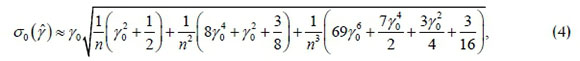
where γ₀and n are the IC γand sample size respectively.

Note that the LCL and UCL are functions of n. For the existing synthetic- γchart, which adopts fixed sample sizes, there is only one pair of (LCL, UCL). However, if variable sample sizes are adopted - for example, small and large sample sizes (ns and nL) - there will be a pair of (LCL, UCL) for ns and another pair of (LCL, UCL) for nL. In addition, VSS charts involve lower and upper warning limits (LWL and UWL) to establish the warning region, where, similar to the LCL and UCL, they are also functions of n. Thus, if two levels of sample sizes are adopted (ns and nL), there will be two pairs of (LCL, UCL) and two pairs of (LWL, UWL) - i.e., one pair of (LCL, UCL) and (LWL, UWL) for ns, and another pair of (LCL, UCL) and (LWL, UWL) for nL. Furthermore, both the warning and the control limits are asymmetric limits. This results in a significant increase in the computational effort to design the chart because of the larger number of charting parameters. It also results in a difficulty during implementation and interpretation, as the samples need to be plotted against different pairs of limits [8].

Thus the approach by Castagliola et al. [8] is adopted: instead of directly monitoring of the i^th subgroup , the transformed statistics Ti are monitored instead. The statistics Ti are defined as

where a,b > 0 and c are parameters that depend on n(i) and γ₀. Here, n(i) is the sample size of the 7^th subgroup. The parameters (a,b,c) can be estimated as

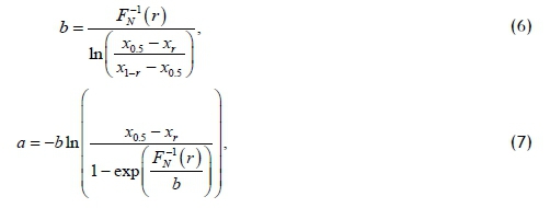
and

 

where are the quantiles for the distribution of , and is the inverse standard normal distribution. Note that (.) is the inverse cumulative distribution function (cdf) of where being the inverse cdf of the non-central t distribution.

Castagliola et al. [8] have shown that, for r e [0.01,0.1], the T statistics are well approximated by a standard normal distribution, as r > 0.01 will avoid giving too much weight to the tails of the f distribution, while r < 0.1 will capture enough information from the tails. Through simulations, Castagliola et al. [8] have shown that the Ti statistics follow the standard normal distribution for r e [0.01,0.1]. This is achieved by simulating a large number of f from different values of n and γ₀, computing the Ti statistics based on

different r values between 0.01 and 0.1, and performing an Anderson-Darling test to show that the Ti statistics follow a standard normal distribution for all values of r within that range. In this paper, as in that of Castagliola et al. [8], the intermediate value of r = 0.05 is adopted. However, practitioners can also choose other values of r e [0.01,0.1] for the Ti statistics to follow the standard normal distribution; hence any value of r e [0.01,0.1] will not have an impact. Note that the Ti statistics are only approximated well by a standard normal distribution if the observations of the quality characteristic being monitored are independent and identically distributed normal variates.

 

3 THE VARIABLE SAMPLE SIZE (VSS) SYNTHETIC-^f CHART

The proposed chart works in a similar way to the existing synthetic- γchart, except that the sample size is varied at two levels, as shown in Figure 1.

Figure 1 shows that the conforming region is separated into the central and warning regions. When -W < T_i < W , the sample belongs to the central conforming region, while when W < T_i < K or -K < T_i < -W , the sample falls in the warning conforming region. When t > k or t_i <-k , the sample is non-conforming. The samples that fall in the central conforming, warning conforming, and non-conforming regions are denoted as 0_C ,0_Wand 1 respectively.

The sample size n (i ) of the 7^th subgroup depends on the region in which T_i-1falls. If T_i-1falls in the central conforming region, then n (i) = n_S; but if T_t-1falls in the warning conforming region or the non-conforming region, then n (i) = n_L.

Let

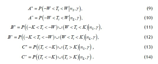
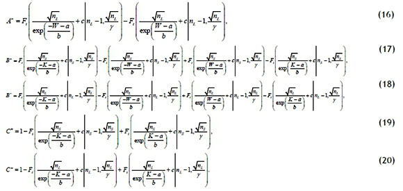
The probability A* is obtained as follows:

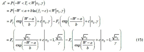
where F_f(.) is the cdf of γand F_t(.) is the cdf of the non-central t distribution. Castagliola et al. [6] have shown that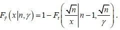

Similarly, the probabilities can be obtained as follows:

The formulae for the average run length (ARL), standard deviation of the run length (SDRL), expected average run length (EARL), and average sample size (ASS) will be developed using a Markov chain approach. The states of the Markov chain are defined based on L consecutive samples; thus there will be a total of ( 2L +1) IC states that are transient and one OOC absorbing state. The OOC absorbing state refers to the state where CRL < L .

For L = 2, the transient states are defined as

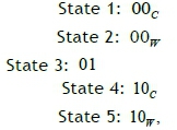
where 0 denotes the conforming region, while State 6 will be the absorbing state. For L > 3, the transient states are defined as

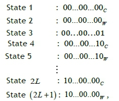
while State ( 2L + 2 ) will be the absorbing state.

A ( 2L +1) χ ( 2L +1) matrix that consists of the transition probabilities among the transient states, as defined

in the previous paragraph, can be obtained. This transition probability matrix is denoted as Q . For L = 2 , Q can be obtained as follows:

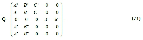
For L > 3, Q is a (2L + 1)χ( 2L +1) matrix with all elements zero, except:

1. For the first row, Q (1,1) = A⁺, Q (1,2) = B⁺, Q (1,3) = C +.

2. For the second row, Q(2,1) = A",Q(2,2) = B~,Q(2,3) = C^-.

3. For the third row, Q (3,4) = A" ,Q (3,5) = B^-.

4. For rows i, where i = 4,...,(2L -1), if i is even, Q(i,i + 2) = A⁺,Q(i,i + 3) = B⁺, while if i is odd,

Q +1) = A",Q (i,i + 2)= B-.

5. For row (2L) , Q(2L,1) = A⁺,Q (2L,2) = B⁺.

6. For row (2L +1), Q (2L +1,1) = A',Q (2L +1,2)= B- .

The transition probability matrix can then be obtained as follows:

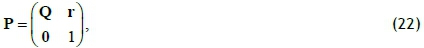
where Q is the (2L + 1)χ(2L +1) matrix as shown in the preceding paragraph, r = 1 - Ql with 1 being a (2L + 1)χ 1 vector of ones, and 0 is a 1χ(2L +1) vector of zeros. Note that state (2L + 2) of P in (14) is the OOC state.

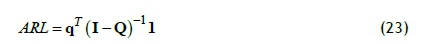
The ARL and SDRL can then be computed as

and

where q is the (2L + 1)x 1 vector of initial probabilities for the transient states, I is the (2L + 1)x(2L +1) identity matrix, and 1 is a ( 2L +1) x 1 vector of ones. For a zero-state condition, except for the 3^rdelement of q which is one, all other elements are zeros. This paper will design the proposed chart based on the zero-state condition.

To calculate the OOC ARL (ARL ) and OOC SDRL (SDRL₁), γ = γ₁= τγ₀ (τ> 1) is substituted into Equations (15) to (20), where γ₁is the OOC γand τis the shift size, to obtain the OOC Q from Equation (21). To compute the IC ARL ( ARL₀) and SDRL ( SDRL₀), γ = γ₀is substituted into Equations (15) to (20) to obtain the OOC Q from Equation (21 ). The ARL₁and SDRL₁are then calculated by substituting the OOC Q into Equations (23) and (24) respectively, while ARL₀and SDRL₀are calculated by substituting the IC Q into Equations (23) and (24) respectively.

The exact value of τis not always known, and without knowing its exact value, the ARL1 cannot be computed. For this scenario, the EARL will be adopted as a performance measure. The EARL does not require the shift size to be estimated as an exact value; instead, it only needs to be estimated as a range

The following shows the computation of the EARL:

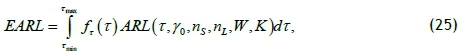
where is the probability density function (pdf) of τ. As in the study of Castagliola et al. [6], τis assumed to be uniformly distributed over . The integral cannot be obtained analytically; thus the Gauss-Legendre quadrature is adopted to solve the integral.

Subsequently, the formula for the ASS will be shown. The ASS needs to be evaluated so that the IC ASS ( ASS0) can be maintained at a specific value, especially when the cost of sampling is of concern to the practitioner.

The formula for the ASS is developed through a Markov chain approach, as proposed by Castagliola et al. [8]. First, P in Equation (22) is transformed into a similar matrix P*, where

From P*, once the process reaches the OOC state (State (2L + 2) ), the process will restart at State 3.

Let be the stationary probability vector of Ρ*, where π _j is the stationary probability for the process to fall in the j^th state, where j = 0,1,...,2L + 2 . π can be computed as follows:

where the matrix R is obtained by deducting 1 from the diagonal elements of the transpose of P* ; then replace the third row of this matrix with ones.

The ASS is then computed as

 

4 NUMERICAL EXAMPLES

This section shows the algorithms to obtain the optimal charting parameters (L*, n*, n_L, W",K* ). Next, the optimal charting parameters ARL1 and SDRL1 for the numerical examples with different values of γ₀,n and τare shown. Furthermore, the optimal charting parameters and EARL1 for different γ₀and n are also shown for the case when τcould not be specified.

Two algorithms are proposed. In the first algorithm, ( L*, n*, n_L ,W *, K * ) is chosen to minimise ARL1, subject to constraints in ARL0 and ASS0. In the second algorithm, ( L, n*, n*,W *, K * ) is chosen to minimise the EARL instead, subject to constraints in ARL0 and ASS0.

The following are the steps to implement the first algorithm:

1. Specify the values of n, γ₀, ARL0 and τ.

2. Set L = 1.

3. Set n_s = 2 .

4. Set n_L = n +1, where n is the sample size.

5. Obtain (W,K) so that ARL₀ = ξand ASS0 = n, by solving Equations (23) and (28) with γ = γ₀. Note that ξis determined by the practitioner.

6. With the current combination of (L,n_S,n_L,W,K), compute ARL1 and SDRL1 from Equations (23) and (24) respectively, with γ = τγ₀.

7. Increase n_Lby 1.

8. Repeat Steps 5 to 7 until n_L = n_max, where n_maxis determined by the practitioner based on the availability of resources. In this paper, n_max = 31.

9. Increase n_Sby 1.

10. Repeat Steps 4 to 9 until n_S = n -1.

11. Increase L by 1.

12. Repeat Steps 3 to 11 until the ARL1 for L+1 is larger than the ARL1 for L.

13. The combination with the smallest ARL1 is the optimal charting parameters (L,n*,n*,W*,K*).

In the second algorithm, (L*,n*,n*,W*,K*) is chosen to minimise the EARL instead. The steps to obtain (L*, n*, n*,W *, K* ) are similar to Steps 1 to 13 in the preceding paragraph, with modifications made for the following steps:

1. Specify the values of n, γ₀, ARL0, v_nand .

6. With the current combination of (l,n_S,n_L,W,K), compute EARL1 from Equation (25).

13. The combination with the smallest EARL1 is the optimal charting parameters (L*,n*,n_L,W',K*).

Table 1 shows the (LL,n*,nL,W',K*), ARL1 and SDRL1 values for n e {5,7,10,15}, τe {1.1,1.2,1.5,2.0} and γ₀ e {0.05,0.10,0.15,0.20}. The ARL0 is set as 370.4. To interpret Table 1, we refer to the combination γ₀ = 0.05,n = 5 and τ= 1.1, which shows that (L,n"*,n"*,W",K") = (28,2,30,1.60,2.19) , with ARL1 = 68.92 and SDRL1 = 92.75.

From Table 1, most of the optimal charting parameters show a large difference between n^*_Sand n^*_L, where all the n* = 2 , while most of the n*_Lare equivalent or close to n_max. A larger n results in smaller ARL1 and SDRL1 values. For example, for γ₀ = 0.05 and τ = 1.1, (ARL_l,SDRL₁ ) = (68.92,92.75) when n = 5, while (ARL₁,SDRL) = (36.64,48.39) when n = 15. Thus a larger n results in a better performance. The improvement is more significant when τis small. A smaller W and a larger K are also observed for a larger n, which translates into a larger warning region but a smaller conforming region.

Similar to n, smaller ARL1 and SDRL1 are observed for larger τ, since a larger shift requires fewer samples to detect the shift. A larger τalso results in smaller L and K. This shows that a smaller conforming region is adopted; but successive non-conforming samples should happen quite close to each other for the process to be considered as OOC. A larger γ₀results in a slight increase in the ARL1 and SDRL1, especially for small shift sizes.

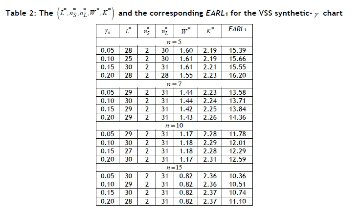
Table 2 shows the and EARL1 values for I =(1,2] by using the second algorithm. Similar to Table 1, the ARL0 is set as 370.4. For instance, for = (1,2] , γ₀ = 0.05 and n = 5 , (L',n'_s, n*_L ,W",K" ) = (28,2,30,1.60,2.19) , with EARL = 15 39 .

Similar to Table 1, there is a large difference between n_Sand n_L. A smaller value of EARL1 is shown for a larger n. A smaller W and a larger K are also observed for a larger n. Overall, a similar trend is observed for Tables 1 and 2

 

5 COMPARISON

The proposed chart is compared with the following γcharts: the synthetic- γ, VSS-γ , VSS EWMA- γ², EWMA- γ²and Shewhart- γcharts.

Table 3 shows the ARL1 values of the proposed VSS synthetic- γchart and the five competing charts, as mentioned in the previous paragraph. The ARL1 values are shown for n e {5,7,10,15}, τ e {1.1,1.2,1.5,2.0} and γ₀= 0.05 , with the ARL0 being set as 370.4. To facilitate comparisons, the relative ARL (RARL), which is the ratio of the ARL1 for the competing chart against the ARL1 for the VSS synthetic- γchart, is shown in Table 3. For instance, for n = 5 and τ = 1.1, the RARL for the Shewhart- γchart is . The proposed chart outperforms competing charts with a RARL that is larger than unity.

From Table 3, the VSS synthetic- γchart shows a smaller ARL1 than the Shewhart- γ, VSS- γand synthetic-γcharts for all n and τvalues. The magnitude of improvement is quite large for small values of n and τ. In particular, comparison with the synthetic- chart shows that the VSS feature results in a significant improvement. For example, for n = 5 and τ = 1.1, the ARL1 = 115.42 for the synthetic- γchart, while ARL1 = 68.92 for the VSS synthetic- γchart. This shows that incorporating the VSS feature results in an improvement of 40.29% in the ARL1 criterion.

However, the VSS synthetic- chart does not outperform the EWMA- ² and VSS EWMA- ² charts for all the shift sizes. With the exception of small shift sizes of τ = 1.1, Table 3 shows that the VSS synthetic-γ chart outperforms the EWMA- ² chart for most cases. This is expected, since the EWMA- ² chart is well-known for its sensitivity to small shifts. However, the VSS synthetic- chart is not as complicated as the EWMA- γ² chart, which makes it more user-friendly for practitioners. Furthermore, the EWMA- γ² chart only shows a better performance for τ = 1.1, while, for other values of τ, the VSS synthetic- γchart shows a better performance. The VSS synthetic- chart outperforms the VSS EWMA- ² chart for moderate and large shift sizes of τ = 1.5 and τ = 2.0 , but is inferior to the VSS EWMA- γ² chart for τ = 1.1 and τ = 1.2 .

Performance in terms of the ARL1 criterion can only be evaluated if τis known. Since τmay not be known in practical applications, EARL1 comparisons are also made. Table 4 shows the EARL1 values of the VSS synthetic- γchart and the five competing charts for n e{5,7,10,15} and γ₀ e {0.05,0.10,0.15,0.20}. Similar to Table 3, the relative EARL (REARL) is provided for ease of comparison, where the REARL is computed and interpreted in a similar way to the RARL.

From Table 4, the VSS synthetic- γchart outperforms the Shewhart- γ, VSS- γand synthetic- γcharts for all values of n and γ₀considered in Table 4. This result is consistent with the comparison based on the ARL1 criterion in Table 3. However, the VSS synthetic- γchart only slightly outperforms the EWMA- γ²chart for n = 5, but does not perform as well as the EWMA- γ²chart for cases with n ε {7,10,15}. By comparison, the VSS EWMA- γ²chart outperforms the proposed chart for all values of n and γ₀considered in Table 4.

 

6 AN ILLUSTRATIVE EXAMPLE

This section shows the implementation of the VSS synthetic- γchart with the example by Castagliola et al.

[8], who have shown that it is not appropriate to use X and S control charts to monitor the process owing to an unstable mean and standard deviation. However, Castagliola et al. [8] conducted a regression analysis that showed a constant proportionality between the standard deviation and the mean of the process. Thus monitoring γis a good alternative for this process. This section illustrates the monitoring of this process using the VSS synthetic- γchart.

Table 5 (left-hand side) shows the sample mean , sample standard deviation (Sj) and sample S for the Phase-I data, which consist of m = 30 samples, with size n = 5, where

γ_ois estimated as

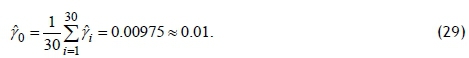
Castagliola et al. [8] showed that the Phase-I data are IC. Thus the f₀in Equation (29) can be adopted.

Next, Phase-II data, which consist of m = 30 samples, are collected, and are shown in Table 5 (right-hand side). Similar to the Phase-I data, the and values of the Phase-II samples are also shown. As the transformed statistics Ti in Equation (5) are monitored in the VSS synthetic- γchart, Table 5 also shows the Ti for each sample.

According to Castagliola et al. [8], it is important to detect a shift of 20% in γ. Thus the chart is optimised to detect a shift of τ = 1.20 . From the methodology in Section 4, for n = 5,γ₀ = 0.01 and τ = 1.20 . From these optimal charting parameters, if -1.58 < T_i < 1.58 , n(i +1) = 2, while if T_i > 1.58 or T_i<-1.58 , n(i +1) = 30 . The sample size for each sample n(i) is shown in Table 5. Since K* = 2.17, the sample is non-conforming if T_i > 2.17 or T_i<-2.17 . The t_ivalues in bold in Table 5 are the samples that are non-conforming. If CRL < 23, the chart will give an OOC signal. Adopting these optimal charting parameters results in (ARL₁,SDRL_l) = (14.02,20.16).

Figure 2 shows the γsub-chart for the Phase-II data. From Figure 2, we can see that there are three nonconforming samples: samples 3, 8, and 19. From Figure 2, CRL₁ = 3, CRL₂ = 5 and CRL₃ = 11. Since all the CRLs are less than 23, OOC signals will be produced at samples 3, 8, and 19.

For comparison, this paper will also show the monitoring of the Phase-II data with the synthetic- γchart without the VSS feature. Similar to the VSS synthetic- γchart, the synthetic- γchart is optimised to detect a shift of τ = 1.20, which results in the optimal charting parameters ( L*, LCL ,UCL ) = (39,0.002217,0.01942 ) . Note that, since the synthetic- γchart adopts fixed sample sizes, there is no need to monitor the transformed statisticsT_i. Instead, γ_{ is monitored directly. Figure 3 shows the γsub-chart for the synthetic- γchart without the VSS feature.

From Figure 3, only sample 9 is a non-conforming sample, with CRL₁ = 9 . Thus sample 9 is an OOC sample. This shows that the synthetic- γchart only managed to detect one OOC sample at sample 9, whereas the VSS synthetic- γchart detected three OOC samples at samples 3, 8, and 19. This shows that the VSS synthetic- γchart improves the performance over the synthetic- γchart.

Figures 2 and 3 can only be obtained if τis known in advance. Since τmay not be known in advance, we also consider the case when τis unknown. By adopting the methodology in Section 4 for n = 5,γ₀= 0.01 and (τ_αία,τ_αβχ) = (1,2], (L,n*_s,n*_L,W\K*) = (23,2,30,1.58,2.17) for the VSS synthetic- γchart, while (L,LCLLjjCLL) = (39,0.002217,0.01942) for the synthetic- γchart, which are the same optimal charting parameters as those for τ = 1.20 . Since the same optimal charting parameters are adopted, the design based on the EARL also gives OOC signals for the same samples as the design based on the ARL.

 

7 CONCLUSION

The synthetic- γchart is attractive to practitioners, as it waits for two successive samples to fall outside the control limits before deciding whether the process is IC or OOC. However, the existing synthetic- γchart is based on fixed sample sizes, where the same sample size is adopted irrespective of the current sample information. To improve the performance of the existing synthetic- γchart, a VSS synthetic- γchart is proposed in this paper to monitor γ. In the proposed chart, the sample size alternates between the small and the large sample sizes, dependent on whether the previous sample is in the central, warning, or non-conforming regions. Formulae to evaluate the ARL, SDRL, EARL, and ASS are developed, and optimisation algorithms to obtain the optimal charting parameters are proposed. Tables of optimal charting parameters are also provided to facilitate a quick implementation of the proposed chart. The optimal charting parameters show that there is a large difference between n_Sand n_L. Thus practitioners are encouraged to adopt a smaller sample size when γis in the central region, and to adopt larger sample sizes when γfalls in the warning or non-conforming region. The proposed chart shows a significant improvement over the existing synthetic- γchart. Furthermore, the VSS synthetic- γchart also outperforms the VSS- γand Shewhart- γcharts for all shift sizes, while outperforming the EWMA- γ¹and VSS EWMA- γ²charts for moderate and large shift sizes. Note that, with the exception of very small shift sizes, the VSS synthetic- γchart shows a better performance than the EWMA- γ¹chart.

 

8 REFERENCES

[1] Coelho, M., Chakraborti, S. and Graham, M.A. 2015. A comparison of Phase I control charts. The South African Journal of Industrial Engineering, 26(2), pp. 178-190.         [ Links ]

[2] Teoh, W.L., Fun, M.S., Khoo, M.B.C. and Yeong, W.C. 2016. Exact run length distribution of the double sampling X-bar chart with estimated process parameters. The South African Journal of Industrial Engineering, 27(1), pp. 20-31.         [ Links ]

[3] Kang, C.W., Lee, M.S., Seong, Y.J. and Hawkins, D.M. 2007. A control chart for the coefficient of variation. Journal of Quality Technology, 39(2), pp. 151-158.         [ Links ]

[4] Yeong, W.C., Khoo, M.B.C., Tham, L.K., Teoh, W.L. and Rahim, M.A. 2017. Monitoring the coefficient of variation using a variable sampling interval EWMA chart. Journal of Quality Technology, 49(4), pp. 380-401.         [ Links ]

[5] Calzada, M.E. and Scariano, S.M. 2013. A synthetic control chart for the coefficient of variation. Journal of Statistical Computation and Simulation, 83(5), pp. 853-867.         [ Links ]

[6] Castagliola, P., Celano, G. and Psarakis, S. 2011. Monitoring the coefficient of variation using EWMA charts. Journal of Quality Technology, 43(3), pp. 249-265.         [ Links ]

[7] Castagliola, P., Achouri, A., Taleb, H., Celano, G. and Psarakis, S. 2013. Monitoring the coefficient of variation using a variable sampling interval control chart. Quality and Reliability Engineering International, 29(8), pp. 1135-1149.         [ Links ]

[8] Castagliola, P., Achouri, A., Taleb, H., Celano, G. and Psarakis, S. 2015. Monitoring the coefficient of variation using a variable sample size control chart. International Journal of Advanced Manufacturing Technology, 80, pp. 1561 -1576.         [ Links ]

[9] Khaw, K.W., Khoo, M.B.C., Yeong, W.C. and Wu, Z. 2017. Monitoring the coefficient of variation using a variable sample size and sampling interval control chart. Communications in Statistics - Simulation and Computation, 46(7), pp. 5772-5794.         [ Links ]

[10] Yeong, W.C., Lim, S.L., Khoo, M.B.C. and Castagliola, P. 2018. Monitoring the coefficient of variation using a variable parameters chart. Quality Engineering, 30(2), pp. 212-235.         [ Links ]

[11] Anis, N.B.M., Yeong, W.C., Chong, Z.L., Lim, S.L. and Khoo, M.B.C. 2018. Monitoring the coefficient of variation using a variable sample size EWMA chart. Computers & Industrial Engineering, 126, pp. 378-398.         [ Links ]

[12] Reh, W. and Scheffler, B. 1996. Significance tests and confidence intervals for coefficients ofvariation. Computational Statistics & Data Analysis, 22(4), pp. 449-452.         [ Links ]

 

 

Submitted by authors 26 Jun 2021
Accepted for publication 15 Nov 2021
Available online 06 May 2022

 

 

ORCID® identifiers
M. Yahaya 0000-0003-1426-7630
S.L. Lim 0000-0003-3554-6874
A.I.N. Ibrahim 0000-0003-4174-6434
W.C. Yeong 0000-0002-0579-6621
M.B.C. Khoo 0000-0002-3245-1127
* Corresponding author sokli@um.edu.my