GENERAL ARTICLES

 

Walk modelling when designing small bus transit networks

 

 

G. Hüsselmann^{I, *, #}; J.H. van Vuuren^I; S.J. Andersen^II

^IDepartment of Industrial Engineering, Stellenbosch University, South Africa. G. Hüsselmann: https://orcid.org/0000-0001-6711-8546; J.H. van Vuuren: https://orcid.org/0000-0003-4757-5832
^IIDepartment of Civil Engineering, Stellenbosch University, South Africa. https://orcid.org/0000-0002-3760-1374

 

 

---

ABSTRACT

Models for the design of public bus transit networks are usually based on the historically observed origin-demand travel patterns of potential passengers. The option of a passenger choosing to walk is, however, not usually incorporated into the design models for such networks. We argue that the absence of this model feature might lead to significant sub-optimality, especially in the design of small public bus transit networks. A novel approach to including this feature in the bus frequency setting aspect of public bus transit network design models is demonstrated in this paper, in which passenger transit modal choices are modelled on the basis of an existing optimal strategy transit assignment model. The newly proposed bi-objective route design and frequency setting models are applied to a realistic case study involving the establishment of a public bus transit system for students on a university campus; and this model implementation is used to gain insight into passenger route choice behaviour, based on individual preferences between walking or using buses. It is shown in the context of this case study that including the option of a passenger walking in the design models for public bus transit networks can affect the efficacy of the final network, especially if the network is small.

---

OPSOMMING

Modelle vir die ontwerp van openbare busvervoernetwerke word gewoonlik gebaseer op histories waargenome reispatrone van potensiële passasiers. Die opsie dat 'n passasier mag kies om te loop word egter gewoonlik nie in die ontwerpmodelle van sulke netwerke geïnkorporeer nie. Ons voer aan dat die afwesigheid van hierdie modelaspek kan lei tot beduidende sub-optimaliteit in die ontwerp van veral klein openbare busvervoernetwerke. n Nuwe benadering tot die insluiting van hierdie aspek in roete-ontwerp en frekwensie-bepalingsmodelle vir openbare busvervoernetwerke word in hierdie artikel gedemonstreer, waarin modale keuses vir passasiersvervoer berus op n bestaande optimale strategie toewysingsmodel. Die nuut-voorgestelde tweedoelige roete-ontwerp en frekwensie-bepalingsmodelle word in n realistiese gevallestudie toegepas in die ontwerp van n openbare busvervoernetwerk vir studente op n universiteitskampus; en hierdie model implementasie word gebruik om insig te verkry in die roete-gedrag van passasiers, gebaseer op individuele voorkeure tussen loop of die gebruikmaking van busse. Daar word in die konteks van hierdie gevallestudie getoon dat die insluiting van die opsie dat n passasier mag kies om te loop in modelle vir die ontwerp van openbare busvervoernetwerke die doeltreffendheid van die finale netwerke noemenswaardig kan beïnvloed, veral as die netwerk klein is.

---

 

 

1 INTRODUCTION

The problem of designing a set of routes in a public bus transit network is commonly referred to as the 'transit network design problem', for which there are a number of variations in the literature. This problem involves (i) designing a set of bus routes, by selecting the order in which bus stops should be traversed along each route, and then (ii) assigning the frequencies with which buses should operate along each of these routes. The solution of this problem is typically guided by the historically observed ' origin-destination' (OD) demand data of potential passengers, as well as the existing road network along which buses are required to travel. Popular objectives adopted during this design process are the minimisation of the passenger travel cost (usually measured in units of time and including waiting time, travel time, and transfer time) and the minimisation of the operational cost of the transit system incurred by the network operator, making this problem inherently bi-objective. It therefore requires design decisions in the form of appropriate trade-offs.

Models in the literature for the design of public bus transit networks do not, however, usually allow for the possibility that passengers might opt to walk instead of travelling by bus if their origins and destinations are relatively close to each other. In this paper, we introduce a novel approach to including the option of walking in the bus frequency setting aspect of the design of a public bus transit network. This is achieved by modelling passenger transit modal choices that are explicitly based on an existing optimal strategy transit assignment model.

In particular, we propose two bi-objective minimisation models to solve each of the two phases of network design separately: (i) the route design phase above, followed by (ii) a bus frequency setting phase. Each of these models is solved using a popular version of the genetic algorithm (GA). These algorithmic implementations for bus route design are applied to a realistic case study involving the design of a small public bus transit system. The approximately Pareto-optimal model solutions computed are used to gain insight into passenger route choice behaviour, based on preferences between walking or using buses. In this way, it is shown that including the option for passengers to walk in public bus transit network design models can affect the final network's efficacy - and the smaller the network, the more pronounced this effect on the network's efficacy.

This article is organised as follows: Section 2 contains a brief literature review focused on the transit network design problem and its various sub-problems. Our model formulations are proposed in Section 3, while our GA implementation is elaborated on in Section 4. Section 5 is devoted to a presentation and discussion of the numerical results returned by the algorithmic implementations in the context of a practical case study. The paper closes with a brief conclusion in Section 6.

 

2 LITERATURE REVIEW

The problem described in Section 1 is a special case of a more general problem, called the 'urban transit network design problem' (UTNDP). In this problem, the goal is to find a configuration of various transit routes and associated bus frequencies that minimises or maximises a pre-selected set of objective functions, subject to various constraints. Typical examples of these objective functions and constraints may be found in [1, 2, 3]. Most of the work on the UTNDP in the literature scalarises the objective functions into a weighted sum, whereas an inherently multi-objective optimisation problem should rather be solved in a Pareto trade-off fashion. The UTNDP is an NP-hard, mixed combinatorial optimisation problem, and Baaj and Mahmassani [4] identified five sources for the complexity of the UTNDP.

According to Ceder and Wilson [5], the planning process for transit networks can be partitioned into a sequence of five distinct steps. These steps are route design, frequency setting, timetable development, bus scheduling, and driver scheduling. The activities associated with these five steps require different independent inputs and yield different outputs. The output of each step (other than the last) serves as the input to the next step. The clear and distinct order, as well as the independence of each of these activities, only exists in theory: in reality they are all intertwined, because decisions made earlier in the sequence will typically have an effect on the activities later in the sequence.

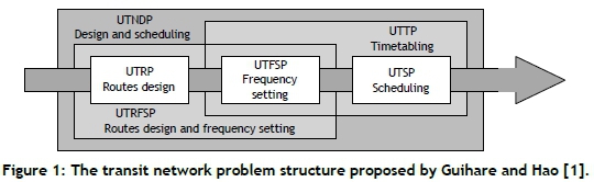
Guihare and Hao [1] proposed a naming convention for the UTNDP facets of the aforementioned planning process. At its core, the UTNDP may be viewed as three different sub-problems, while simultaneously solving two or more of these sub-problems leads to other, higher-level sub-problems. The three core subproblems are the urban transit routing problem (UTRP), the urban transit frequency setting problem (UTFSP), and the urban transit scheduling problem (UTSP). When the UTRP and the UTFSP are, however, solved simultaneously, the result is called the urban transit routing and frequency setting problem (UTRFSP), and when the UTFSP and the UTSP are solved simultaneously, the result is called the urban transit timetabling problem (UTTP). When all three core sub-problems are solved simultaneously, the result is called the UTNDP. A graphical depiction of this partitioning is provided in Figure 1 The focus of this article is on the UTRP and the UTFSP.

 

 

Public transport systems aim to meet the needs of passengers while simultaneously minimising the operational cost of the system [3]. When deciding on the UTNDP objectives to be pursued, both passenger and operator perspectives have to be considered. Most studies in the literature focus on both economic efficiency and service quality during the design of transit systems. The main objectives in the literature can be summarised as maximising passenger benefits, minimising operator costs, maximising total welfare, maximising system capacity, conserving energy, and optimising individual parameters [3]. In the UTRP, the decision variables that are adopted encode bus routes, while in the UTFSP the service frequencies associated with bus routes are the decision variables. The constraints considered in UTNDP instances are mainly associated with a mix between performance requirements and resource limitations [6]. Kepaptsoglou and Karlaftis [3] provide more details on the intricacies of the problems pertaining to network structure, demand patterns, and demand characteristics.

Various solution techniques have been adopted to solve instances of the aforementioned sub-problems, and these techniques may be partitioned into four categories: exact solution approaches, heuristic approaches, metaheuristic approaches, and hybrid approaches [1]. The class of exact solution approaches contains exhaustive searches and mathematical programming solution techniques, but these are only computationally feasible for small network instances [1]. Some of the earlier solution approaches adopted for larger networks were heuristics, such as Mandl's approach [7]. More recently, metaheuristics have predominantly been adopted to solve instances of the UTNDP and its sub-problems, often yielding high-quality results within reasonable time frames. These metaheuristics can be classified into two classes: trajectory-based metaheuristics and population-based metaheuristics [8].

Zhao and Gan [9] proposed an aggregated metaheuristic UTNDP solution approach in 2003, incorporating the application of an integrated simulated annealing, tabu, and greedy search algorithm, as well as a greedy search algorithm and a fast hill climbing algorithm. The two objectives pursued were the minimisation of the number of bus route transfers incurred by passengers and the maximisation of service coverage by the routes.

In 2004, Fan and Machemehl [10] wrote a report containing various detailed descriptions of the UTRP and its intricacies. They cast the UTRP as a multi-objective non-linear mixed-integer model, but weights were assigned to each objective. The weighted sum of the objectives was minimised, accounting for total passenger travel time, the total number of buses required, and unsatisfied demand cost. Their proposed approach to a solution had three phases: an initial candidate route set generation procedure, a network analysis procedure for evaluating performance, and a metaheuristic search procedure. Five metaheuristic search procedures were employed.

Fan and Machemehl [6, 10], Chakroborty [11], and Mumford [12] cited examples in which GAs had been applied to instances of the UTRP, and reported great success in finding high-quality solutions. John, Mumford and Lewis [13] applied the celebrated non-dominated sorting genetic algorithm II (NSGA II) framework in 2014 to solve the UTRP, cast as a multi-objective optimisation problem, and used intuitive graph-theoretic principles to model the problem. John's dissertation of 2016 [14] contains extensive details on his approach to solving instances of both the UTRP and the UTFSP.

When solving instances of the UTFSP, an important component is the passenger assignment sub-problem in which, according to the service frequencies set for each bus route, passenger flows have to be assigned to the appropriate bus routes in the transit network. A popular transit assignment model adopted in the context of the UTFSP is the optimal strategies assignment model proposed by Spiess and Florian [15] in 1989. Martínez, Mauttone and Urquhart [16] used this optimal strategies assignment model to solve instances of the UTFSP. They formulated a mixed-integer linear programming model for the UTFSP, and solved it to optimality for small instances. For larger instances, they advised that a metaheuristic be applied, and they chose to implement a tabu search in this respect.

 

3 MODEL FORMULATIONS

A bus route set is required to establish an instance of the UTFSP, and therefore the output of the UTRP, within the same context, serves as input to the UTFSP. When designing a transit system requiring both routes and frequencies, these two problems should be solved either successively or simultaneously, with the latter incurring a larger computational burden. When designing bus routes and bus frequencies for small transit systems, walking may play a significant role, as argued in the introduction, because a passenger may choose to walk instead of waiting for a bus to arrive, and then potentially not always have direct origin-destination routes available. The option of passengers walking has not yet been incorporated into any UTFSP models in the literature. Spiess and Florian [15], however, mentioned that their model might be extended with the inclusion of walk arcs, thus making provision for walking. We incorporate their model extension in the remainder of this article. The model formulations of the UTRP and the UTFSP in this section are inspired by the graph-theoretic modelling approach proposed by John [14].

3.1 UTRP model

We make a number of standard assumptions in our UTRP model formulation. In particular, we assume that there are sufficient vehicles on each bus route so that demand can be satisfied. Bus frequencies are not considered as decision variables, but are instead assumed to be fixed at ¹ [12, 13] - i.e., one bus every ten minutes. Moreover, we adopt the standard assumption from the literature that each bus is assumed to traverse its assigned route, reversing its direction each time a terminal bus stop is reached [13]. Another standard assumption is that a transfer penalty of five minutes is incurred each time a passenger needs to make a transfer, which corresponds to a frequency of ¹ [14]. It is also assumed that the distance matrices, passenger demand, and expected travel time are symmetrical [12]. The passenger demand is assumed to be fixed over time, with each passenger's route choice being determined by the shortest travel time, regardless of transfers. The passenger travel time consists only of in-vehicle travel time and transfer time [12]. Finally, we assume that the locations of bus stops have been determined beforehand, as is the case in most UTRP instances.

We model the road network on which an instance of the UTRP should be solved by an edge-weighted graph G = (V,£), where V = [v_lt ...,v_n] is a set of vertices representing the required bus stops and £ = [e₁, ...,e_m] is a set of edges, each of which is incident with two vertices in V. The edges in £ represent shortest-time direct road links between pairs of vertices in G (in other words, the edges do not contain any intermediate bus stops). The weights of the edges of G are captured in an n x n weight matrix W, representing the travel time measured in minutes [17]. Moreover, an n x n demand matrix D is also associated with G. This matrix contains, as its entry in row i and column the passenger travel demand from vertex v_tto vertex _Vj.

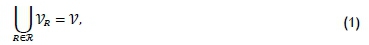
A transit route is defined as a simple path in G, which is represented by an (ordered) sequence of distinct vertices of G, each successive pair of which is adjacent in G. Such a transit route contains no loops or repeated vertices. Let G_R = (V_R,£_R) be the subgraph induced in G by the vertices that appear in a set of transit routes _R. Such a set of transit routes is considered to be an infeasible solution to the UTRP unless each bus stop is contained in at least one route R e R [13]. The transit route set JR is therefore considered infeasible unless

where V_Ris the set of vertices contained in route R. The smallest and largest numbers of vehicle stops are also specified for each route in J [13]. That is, we require that

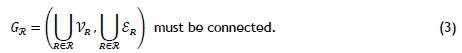
for some natural numbers m_min < m_maK. These limiting values are based on various considerations such as driver fatigue and schedule adherence [9]. Of course, we also require that the subgraph of G induced by all the vertices appearing in a feasible set of transit routes be a connected graph [13]. That is,

Finally, the number of the required transit routes also has to be specified. That is, we specify a requirement of the form

for some natural number r.

In general, passengers are expected to prefer travelling to their respective destinations in the shortest possible time while avoiding the inconvenience of having to make transfers, if possible. The length of a shortest-time path for any OD pair v_i,V_je V along a transit route set l is denoted by a_v._¡Vj(R), and is measured in minutes; it can, of course, be computed using Dijkstra' s well-known shortest-path algorithm applied to the subgraph G_Rof G. This shortest-time path duration includes both transport time and transfer time (if transfers between different routes in l are required). Mumford [12] measured the passenger (time) cost associated with any route set l as the average travel time (ATT) of all passengers, measured in minutes and expressed as

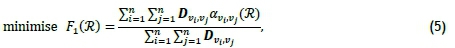
where the numerator captures the total travel time of all passengers and the denominator is the total number of passengers in the system. Mumford [12] also proposed a simple proxy for the operator cost - that is, the sum of the total travel time for a single transport vehicle along each route (in one direction).

This total route time (TRT) may be expressed as

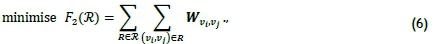
When solving the above model for the UTRP, both of the objective functions (5) and (6) are minimised simultaneously so as to establish a Pareto front, which represents effective trade-offs between minimising passenger cost and minimising operator cost.

3.2 UTFSP model

All of the assumptions of the UTRP model are applicable to the UTFSP model, with the exception of frequencies already being determined. That is, the assumption of ¹ fixed frequencies is not applicable owing to the actual frequencies that can be determined in the UTFSP context. Moreover, instead of the five minutes transfer penalty, the optimal strategies passenger assignment model suggestion of Spiess and Florian [15] is employed to determine the transfer penalties; and the waiting times incurred by passengers, along with the in-vehicle travel times (rather than only the in-vehicle travel times and transfer times considered in the UTRP model) are taken into account. The novel addition to this model is the inclusion of the option of walking.

Let G_K = (V_R,E_R) be the subgraph induced in G by the vertices in a set of transit routes l produced as output by solving the UTRP. Such a set of transit routes, which serves as input to the UTFSP, is assumed to be feasible in terms of containing all the bus stops present in the road network and inducing a connected graph, corresponding to constraints (1) and (3) respectively.

The supply side of the transit network is expressed by an expanded directed graph of the transit network, denoted by G'_R = (V'_R,E'_R), where V'_R includes all the vertices (bus stops) in the road network G, as well as additional transit vertices corresponding to each vertex present in the transit route set l. These vertices are labelled by assigning unique alphabetical letters to each route and attaching each route's letter to the bus stop number present in the specific route, making each transit vertex distinguishable from the others. An example of transit vertices is provided in Figure 2 denoted by A1 and A2. The set of transit vertices is denoted by V_T, with V'_R=VuV_T. The arcs between vertices in V_Tare called transit arcs, denoted by £_T, and represent the bus routes. Transit arcs represent the movement of buses between bus stops, requiring of course that a bus route be available to service the line. The cost (measured in minutes) incurred by travelling from bus stop i e V to bus stop j e V is captured by the weight matrix entry w_ij- e W. Furthermore, arcs directed from vertices in V to vertices in V_Tare called boarding arcs, representing passengers boarding buses, and are denoted by £_B. Arcs directed from vertices in V_Tto vertices in V are called alighting arcs, representing passengers alighting from buses, and are denoted by £_A[16]. Walk arcs, denoted by £_w, are also included in the model, owing to it being a viable option for passengers to walk in smaller transit networks where the distances between bus stops are relatively short and the bus frequencies on routes are perceived to be too low. The sets of transit, boarding, alighting, and walk arcs are therefore subsets of £'_R= £_TU £_BU £_AU £_w.

Figure 2 illustrates the different types of arcs mentioned above in the context of a small example graph, G₁, consisting of only two vertices, 1 and 2. A bus route connecting vertices 1 and 2, denoted by R₁ = {{1,2)}, is applicable in this hypothetical case. Figure 2(a) contains the road network, corresponding to G₁ whereas Figure 2(b) contains the subgraph induced by the route J₁, namely (G₁)R₁, in which the bus route is represented by a transit arc. Figure 2(c) contains the expanded transit network (G1)'R₁ in which the route R₁is represented by vertices A1 and A2.

In essence, the entire transit network is modelled as a graph containing arcs, each characterised by a nonnegative travel cost (measured in minutes), and a service frequency, called a cost-frequency pair [15]. Boarding, alighting, walking, and being in transit are therefore no longer components that are considered separately, but find their relationships with one another expressed in the expanded transit network graph G'_R. The costs associated with the transit arcs £_Tare the on-board travel times between bus stops, as specified in the weight matrix W of §3.1, and the frequencies of these arcs are set to oo, indicating that once a passenger is present on one of these arcs (in transit on a bus), there is immediate service. Boarding arc i e £_Bis assumed to exhibit a cost of six seconds, representing the time a passenger takes to board the bus. The frequency of boarding arc i e £_Bis set to the route frequency f_tassociated with route R_t, indicating that a passenger has to wait until the boarding arc is served prior to boarding the bus. The frequencies f_t e T assigned to each route R_teJl are the decision variables in this model, and each frequency f_tcan take as value a member in the predefined set 0 = {} - the same discretisation as that adopted by Martínez et al. [16].

The alighting arcs in £_A are associated with an alighting time of six seconds, representing the time a passenger takes to alight from a bus. The frequencies associated with these arcs are set to o , representing the fact that once a bus has arrived at a bus stop, a passenger can immediately alight (i.e., does not have to wait for service), as opposed to the case of boarding. The assumption is made that a penalty factor of three times the bus transit time w_ijis imposed when a passenger chooses this alternative, as opposed to travelling by bus, when transitioning between bus stops. However, this assumption is only applicable to small transit networks, and should be adjusted when considering transit networks in which bus stops are located further away from one another. Alternatively, this model feature could be disabled by assigning a very large number as a penalty factor, making the option of walking unattractive to passengers. Figure 3 illustrates how these cost-frequency pairs are assigned to each of the respective arc types mentioned above.

Having established the transit network, the demand side can be addressed by applying the optimal strategies assignment model [15] to the transit network, thereby determining the average travel time for passengers between bus stops i and denoted by u_v._¡v.. This model functions under the core assumption that passengers have a set of attractive lines that they can use to reach their destinations, and that they are distributed along these attractive lines based on the proportion of the lines that are serviced first by buses. Details of the working of the optimal strategies assignment model may be found in [15]. This assignment model also assigns passenger volumes and flows throughout the transit network.

The two objective functions that are minimised simultaneously are passenger cost and operator cost. The first objective function, measuring the average expected travel time (AETT) of passengers in minutes, may be expressed as

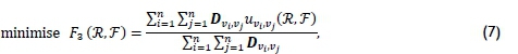
where u_Vi,Vj(R.,F) denotes the expected travel time (measured in minutes) for a passenger travelling from origin i to destination calculated according to the optimal strategies transit assignment model described above [15].

The operator's cost, on the other hand, is the total cost incurred by maintaining the service frequencies along each route. This is measured in terms of the total buses required (TBR) to maintain the frequencies along each route in the route set R. The number of buses required for any particular route is calculated by multiplying the desired frequency of the route by the total round trip time of the route. The round trip time is calculated by doubling the route length (measured in minutes) [4]. The goal of minimising the TBR may therefore be expressed mathematically as

The only constraint applicable to this model occurs when the operators require that the bus frequency along each route be between minimum and maximum acceptable values, denoted by f_minand f_max respectively. This constraint is expressed mathematically as

When solving the UTFSP model above, both objective functions (7) and (8) are minimised simultaneously in order to establish a Pareto front representing effective trade-offs between minimising passenger cost and minimising operator cost.

The route set R remains constant in the UTFSP, and another instance of the UTFSP is generated each time the route set R is altered. The transit assignment model also has to be resolved each time any of the UTFSP frequencies change, owing to the inter-connectedness of the various modelling objectives in the entire transit system.

 

4 MODEL IMPLEMENTATIONS

Population-based approaches are more commonly adopted than are trajectory-based approaches to solve instances of the UTRP, with GAs most frequently being applied as a solution methodology for the UTRP, often leading to very high-quality solutions [2, 12]. We therefore chose a GA to solve the UTRP model of §3.1. The specific GA variant adopted was the NSGA II [18]. This algorithm was also adopted to solve instances of the UTFSP model of §3.2. We implemented the algorithm in the programming language Python.

4.1 Model decision variables representation

The main NSGA II implementation challenge encountered when solving the UTRP model (1)-(6) arose from the fact that routes are not scalar values or vectors of fixed length, but rather vary in length, based on the number of vertices they contain. This challenge may be overcome by using lists as the data type for decision variable representation. The transit route set RR = {R₁,R₂,R₃} would, for example, be represented in this manner as a list of three lists: R₁ = (1,4,5,7,9,8), R₂ = (4,2,3), and R₃ = (9,7,5,6,1). When solving the UTFSP model, a simple vector of length |R| may be used to represent the route frequencies T. For example, would be a possible frequency set for the aforementioned route set RR.

4.2 The initial candidate solution set generation procedure

An initial feasible solution to the UTRP model (1)-(6) was generated by determining the shortest paths between all pairs of vertices and then trimming this list by removing the paths containing more than m_max vertices or fewer than m_min vertices, thus ensuring that each route satisfied constraint (2). A total of r routes were selected randomly from this set of shortest paths and tested for feasibility in terms of constraints (1)-(4). An initial feasible solution to the UTFSP model (7)-(9) was generated by uniformly sampling \l\ frequencies from the pre-specified set with replacement, ensuring that all of the frequencies fell between f_minand f_maxinclusive.

4.3 Network analysis procedures

The ATT objective function (5) of the UTRP model was evaluated by generating an expanded network. This was achieved by inserting additional edges between transfer points in the route set l with an associated cost of five minutes. A more detailed explanation of this expanded network is provided by John [14]. This expanded network could then be used to determine the shortest paths between all pairs of vertices v_i,v_J and each shortest path's cost, measured in minutes. This cost was the a_vIvJ. value associated with the route set J . The TRT objective function (6) of the UTRP model was evaluated by simply adding together the distances of the routes in route set J .

A common network analysis metric involves measuring the number of transfers that passengers have to make while travelling from their origins to their respective destinations. This is expressed in the form of the percentage of demand satisfied without transfers, with one transfer, and with two transfers, while any number of transfers more than two is regarded as unsatisfied demand. This analysis was carried out by counting the number of transfers required for each OD pair, grouping the demand according to each of the aforementioned categories, and dividing these values by the total demand.

The underlying transit assignment problem had to be solved in order to evaluate the AETT objective function (7) of the UTFSP model. The optimal strategies assignment model [15] was employed for this purpose, to determine the u_vi._vj.-values for each v_t,Vj pair, given a route set l and a frequency set F. The walk arcs were considered when applying the optimal strategies assignment, thus giving passengers more flexibility in their route choices.

4.4 NSGA II implementations

The NSGA II employed in this article to solve instances of the UTRP incorporated the initial candidate solution set procedure and network analysis procedure described above, and guided the successive generations of solution populations to converge towards a set of high-quality non-dominated solutions. The crossover operator employed was the same as that of Mumford [12], according to which a route in one parent route set is selected randomly as the seed for an offspring solution, and a second route is chosen from another parent route set that has one vertex in common with the offspring, and that also contains the maximum number of vertices that have not yet been included in the offspring solution. This selection approach is alternated between the parent solutions until r routes have been included in the offspring solution. It is possible, however, that infeasible solutions will thus be generated, and so the repair strategy proposed by Mumford [12] was employed in an attempt to recover feasibility. This was achieved by attempting to insert missing vertices into the transit network by joining them to an adjacent terminal vertex, if possible. If such a repair is not possible, the crossover procedure is repeated afresh until a feasible solution is generated.

Three mutation operators are employed: an exchange operator (proposed by Mandl [7]), an add vertex procedure, and a delete vertex procedure (both proposed by Fan and Mumford [19]). The exchange operator entails randomly selecting two routes in a route set that contain at least one common vertex, after which the parts on either side of a randomly selected common vertex are recombined with the other route's counterparts. Two outcomes are possible, and if the first proves infeasible, the other is performed. Repairs are attempted after each infeasible mutation. If the mutation remains infeasible, all other possible exchanges are attempted for the same offspring. The procedure is terminated when all route combinations have been exhausted without having found a feasible mutation, whereafter the mutation procedure is discarded, and the offspring remains unmutated. The add-vertex procedure involves adding an adjacent vertex randomly to one of the terminal vertices, where possible, without breaking feasibility. The delete-vertex procedure, on the other hand, involves randomly deleting a terminal vertex, once again subject to constraints (1 )-(4), and helps to decrease the TRT operator cost.

The crossover and mutation probabilities were determined empirically as 0.6 and 1 respectively. It is interesting that these values did not conform to the norm of higher crossover probabilities and lower mutation probabilities. These values were nevertheless found to yield the best performance. Furthermore, a population size of 300, along with an evolution over 300 generations, were determined empirically to perform the best in the contexts of a number of small UTRP model instances.

When solving instances of the UTFSP, the above initial candidate solution set procedure, as well as the network analysis procedure, is employed to guide the search for high-quality non-dominated solutions according to the NSGA II framework. Single-point crossover is employed by randomly selecting a frequency position in the decision variable, and then exchanging the corresponding segments in the parents in order to create two new offspring solutions. A bit-flip mutation variant is employed, according to which a frequency entry is changed to a value in 0 one position either above or below the current frequency, with equal probability. When the frequency value is the first entry in 0 and has to be decreased, the last entry is chosen; and vice versa when the last position in 0 is applicable. A suitable value for the crossover probability was determined empirically as 0.7, and a mutation probability of was selected, following John [14].

4.5 Validation of algorithmic implementations

The aforementioned NSGA II implementations were validated by comparing their output with documented solutions to a popular benchmark instance for the UTRP - Mandl's Swiss network [7]. This instance was previously also employed for comparison purposes by Mumford in 2013 [12] and by John in 2016 [14]. As can be seen in Figure 4(a), the attainment front returned by our NSGA II implementation performed satisfactorily, dominating all of the solutions of Mumford, and performing similarly to John's implementation - even dominating a few of his solutions. Not many UTFSP benchmark instances have been cast in a multi-objective context as was done by John [14], and so his UTFSP results were considered exclusively for validation purposes. The route set associated with the smallest operator cost discovered by John [14] was R₀ = [(4,3,1),(13,12),(8,14),(9,10,12),(9,6,14,7,5,2,1,0),(10,11)}, which attained an ATT of 13.480 minutes and a TRT of 63 minutes. As can be seen in Figure 4(b), our NSGA II implementation performed similarly to the route sets computed by John when we assumed a walk factor of 100, with the small deviation being ascribed to our assumption that a boarding and alighting cost of six seconds would be incurred. When, however, a walk factor of 3 was assumed (no walk times are available for the Mandl [7] benchmark instance), it was observed that, at low frequencies, some passengers would prefer to walk instead of using the available buses. This followed from the improvement in the non-dominated front over the attainment front returned for a walk factor of 100.

 

5 A REAL-WORLD CASE STUDY

The above algorithmic implementations were finally applied to a special real-world case study involving the Matie Bus in Stellenbosch to demonstrate the considerable effects of including the option of passengers walking when designing a small public transit network. The Matie Bus is a transport service that Stellenbosch University provides to its students [20]. The focus of the service is to provide transport to students between parking lots and lecture venues on the campus periphery, and lecture venues located centrally on campus. It is shown in this section that an effective redesign of the routes of this bus service could lead to a larger number of students being serviced, even when accounting for the possibility of students preferring to walk.

5.1 Bus stop locations

The day shuttle of the Matie Bus currently services six bus stops between 07h00 and 17h30, Mondays to Fridays. These bus stops are described in the appendix. Recently, Klink [21] published data that were gathered in 2019 about movements along different modes of transport on the campus of Stellenbosch University. He used 44 custom-built Bluetooth-enabled sensors to observe unique identification codes for mobile devices that had Bluetooth enabled. The data revealed the movement of both motorised and non-motorised transport users in terms of volume and spread, and were filtered into OD demand matrices for each hour of the day. These OD demand data were used in this case study. The locations of the 44 Bluetooth sensors were aggregated into ten zones, clustered according to common zoning attributes such as commercial, educational, recreational, or residential. We subsequently decided on alternative locations for bus stops in order to satisfy travel demand between all pairs of zones. These bus stops are labelled 0-9 in Table 3 in the appendix. The corresponding OD demand data may be found in Table 4 in the appendix.

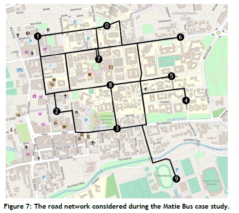
Thereafter we determined the allowable road links that could be considered in an instance of the UTRP as possible edges to be traversed by buses. The reasoning followed during this choice was that the main attraction types are commercial, educational, and recreational, and that all residential areas should be allowed direct access to these attractions. Therefore, no edges exist between the bus stops of residential zones; instead there are edges between the bus stops of non-residential zones and all other bus stops. This road network can be represented as a graph of order 10 and size 36, as illustrated in Figure 7 in the appendix.

5.2 The input data

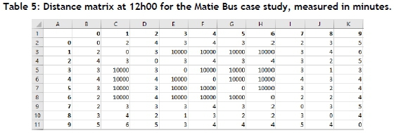
The traversal times associated with road links in the transport network of the Matie Bus are a function of time and traffic density, and can be estimated by using satellite technology [17]. In order to obtain a good approximation of the required distance matrix W, the 12h00 off-peak period was chosen for data gathering purposes, as this period is representative of other periods during a weekday. Estimated travel times were gathered from Google Maps [8] during the 12h00 off-peak period between all of the pairs of the proposed bus stop locations. The resulting weight matrix W is shown in Table 5 in the appendix.

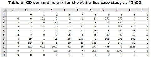
Once a suitable route set had been established for the Matie Bus transportation network, frequencies (or buses) could be assigned to each route so that sufficient provision was made for the demand along the routes. In order to establish a UTFSP model instance to determine these frequencies, an appropriate route set should be chosen from the non-dominated solutions that are obtained when solving the corresponding UTRP model instance. Thereafter, the corresponding UTFSP instance has to be solved for a specific time instant in respect of its own OD demand matrix for that specific instant. The OD demand matrix for 12h00 was chosen for this purpose, and is shown in Table 6 in the appendix.

When choosing the desired number of stops along a route, it was noted that lectures start on every hour of the day from 08h00 to 17h00 inclusive, and that students often have to be transported between different venues for these lectures. Lectures typically end 45-50 minutes after the hour, and so only 10-15 minutes are available for this transportation. The routes should therefore preferably not be more than 10 minutes in length; but if a route is too long, this problem can be remedied by setting the frequencies appropriately once the bus routes have been established. The number of stops was consequently set at two to six per route, allowing the algorithm to find a high-quality set of routes within this range. We specified that eight bus routes be sought in order to accommodate a sufficient service coverage. This number is also the maximum number of buses typically considered when solving Mandl's [7] benchmark instance, which is similar in size.

5.3 Numerical results

The case study was performed by providing the data described in the previous section as input to the NSGA II of §4.4. The route sets recommended by the algorithm are discussed briefly in this section. Figure 5(a) is a graphical representation of the non-dominated attainment front in objective function space from which a decision-maker can make a subjective trade-off selection for implementation purposes. The route set achieving the smallest ATT is considered for implementation purposes because of the limited time available to transport students between lectures. For this to be a viable option, however, the operators should be able to maintain the route set. The TRT associated with the route set determines its viability in this sense, and so this is where a trade-off has to be made. An assumption is made that an ATT of three minutes and 25 seconds provides a sufficient service level in the UTRP context; but it should be kept in mind that the AETT will increase for any solution as soon as waiting times for buses are taken into consideration. The solution adhering to this requirement with the closest ATT is therefore chosen as the recommended route set, indicated in Figure 5(a) by the label A. This solution achieves an ATT of three minutes and 23 seconds and a TRT of 40 minutes. The route set corresponding to Solution A in Figure 5(a) is J = [(5,7,2,8,3,9),(1,7),(7,6),(4,8,5),(7,0),(7,8),(1,0),(2,1,0,6,8,5)}. This route set is anticipated to enable students to reach their respective destinations within the time constraints imposed when transitioning between lectures.

A full route set evaluation for solution A in Figure 5(a) further yields transfer percentages of 95.21 per cent of demand fulfilled with no transfers, and 4.79 per cent with one transfer. According to Chakroborty [11], this route set would be classified as a good route set because it satisfies all transit demand, with a large percentage of the demand being satisfied by direct connections.

Route set A in Figure 5(a) was subsequently taken as input for the UTFSP instance of the Matie Bus case study. It was decided that the routes should be kept constant throughout the day because disruptions caused by variations in the route configuration could confuse the student passengers. The frequencies of buses travelling along these routes can, however, be altered for different times of the day in order to accommodate fluctuating demand. The inclusion of walk arcs in the UTFSP model was discussed in §3.2. A walk factor of 3 was assigned in §4.4 to these walk arcs in the context of a small network (Mandl's Swiss network) [7]. This assumption was required because no walking times were available for Mandl's benchmark instance, and neither were geographical data available from which these times could be determined. For the Matie Bus case study, however, the geographical locations of the bus stops could be used in conjunction with data retrieved from Google Maps [8] to determine the walking times between these stops. The walking times matrix thus generated is shown in Table 7 in the appendix.

The attainment front achieved by the NSGA II of §4.4 can be seen in Figure 5(b) for the 12h00 UTFSP instance, corresponding to the demand matrix in Table 6 in the appendix. For this instance, the set of possible frequencies was taken as 0 = , similar to that employed by Martínez et al. [16]. A solution from the non-dominated front returned by the NSGA II of §4.4, taking into consideration walk arcs, was chosen instead of the non-dominated front corresponding to the omission of walk arcs, thereby facilitating better decisions that were based on more accurate information. It was decided for the small network of the case study, and the associated short travel times of the buses, that it would make sense to select the frequency set corresponding to the best AETT objective function evaluation. This solution is denoted by the label B in Figure 5(b), for which the objective function evaluation results in an AETT of 6.185 minutes when no walk arcs are included, and an AETT of 5.37 minutes when walk arcs are included, along with a TBR of 14.333 buses. The corresponding frequencies with which buses are assigned to routes is . 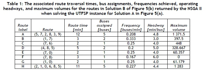The number of buses required is rounded up to the nearest integer, thus ensuring that the minimum required frequency is indeed met. For each route in the route set labelled A in Figure 5(a), the route time, the number of buses assigned to the route, the bus frequency assigned to it, and the headway operating along the route are shown in Table 1

When an integer number of buses is assigned to bus routes, however, the actual frequency of buses operating along each route differs from that returned by the NSGA II of §4.4. Therefore, the AETT was recomputed after the actual number of buses had been assigned to each route (as depicted in Table 1 to achieve a more accurate AETT estimate, resulting in an AETT of 4.443 minutes when no walk arcs are included, and an AETT of 4.288 minutes when walk arcs are included, along with a TBR of 18. The AETT measured when walk arcs were included and that when walk arcs were omitted only differed by a few seconds, because the frequencies were set high enough so that passengers would prefer to use bus transport rather than walking.

When considering the maximum passenger volume flow for the routes labelled A to H in Table 1 it is interesting to note that, when the frequencies were initially set, routes E and F were assigned the smallest discretised frequency in the set 0 - namely, - while all the other routes were assigned the largest discretised frequency in the set 0 - namely, . It is natural to expect that, when the minimum AETT is computed in the context of the UTFSP, all of the frequencies should be set to the highest possible value. In this case, however, the elegance and power of multi-objective optimisation are elucidated, in that the other objective at play, the TBR, is also minimised, albeit without a loss in the quality of the AETT objective. Table 1reveals that these specific routes, E and F, experience maximum passenger flows of 60.357 and 0 respectively, indicating in fact that very few passengers use route E, and no passengers at all use route F.

Table 2contains the non-zero volumes of the walk arcs in the transit network, indicating that passengers prefer to walk between vertices i?₀and i?₇and between vertices i?₇and 1¾. These are exactly the bus stop vertices covered by routes E and F. Although the frequencies may have been set at their maximum values by the NSGA II of §4.4, it became clear that the additional buses and increased frequency would decrease a passenger's travel time, and so the frequencies were set low by the algorithm along these routes to avoid unnecessarily wasting additional buses. Although experiencing a small maximum volume, as shown in Table 1 route G serves the demand flowing between the vertices of the bus route, instead of passengers choosing to walk.

Owing to the rounding up of bus assignments, one bus was assigned to each of routes E and F. It is anticipated, however, that the decision-maker might not consider it beneficial to assign any buses to these routes, as they would serve little, if any, demand. With the removal of routes E and F, a final recommended route set, together with its accompanying bus assignments, is presented in Figure 6 The performance of this solution is an AETT of 4.83 minutes when no walk arcs are included, and an AETT of 4.321 minutes when walk arcs are included, along with a TBR of 16. The final solution performs satisfactorily with respect to servicing passengers with an AETT of under 10 minutes (in fact, even below five minutes), and this is achieved by assigning 16 buses to six different routes.

 

6 CONCLUSION

The results of the previous section reveal the importance of taking the option of walking into account when there are relatively small distances between bus stops. For the small network case of §5, the application of walk arcs was demonstrated, and an analysis of the usage of these arcs revealed insight into anticipated passenger behaviour that otherwise would not have been uncovered. These insights could help decision-makers to design more cost-efficient bus transit networks. This was illustrated by identifying two routes in the route set returned by the NSGA II of §4.4 in the Matie Bus case study of [21] that did not contribute much to the performance of the system based on the UTFSP model results, but were nevertheless selected according to the UTRP model.

Finally, the above observations also illustrate the importance of solving the sub-problems of the UTNDP together. This approach holds considerable value for communities in which the distances between bus stops are relatively small, where the priority of minimising passenger travel time is high, and where additional resources may be used. If, however, no walk arcs are included in the modelling approach, all passengers are effectively forced to make use of the buses, no matter how long the waiting time incurred. This approach can easily be extended to the taxi industry in a South African context, as public transport is typically accompanied by walking. Another application is the possibility of multi-modal logistics, where larger transportation vehicles could be modelled as the buses, in this context, and drones or other small transportation modes could be modelled as walking for the last mile delivery of goods, with the cost of the walk arcs adjusted accordingly. Furthermore, case studies on larger networks could also be conducted in order to build on the work documented in this article.

 

REFERENCES

[1] Guihaire, V. and Hao, J.K. 2008. Transit network design and scheduling: A global review. Transportation Research - Part A: Policy and Practice, 42(10), pp 1251-1273.         [ Links ]

[2] Ibarra-Rojas, O.J., Delgado, F., Giesen, R., and Munoz, J.C. 2015. Planning, operation, and control of bus transport systems: A literature review. Transportation Research - Part B: Methodological, 77, pp 38-75.         [ Links ]

[3] Kepaptsoglou, K. and Karlaftis, M. 2009. Transit route network design problem: Review. Journal of Transportation Engineering, 135(8), pp 491 -505.         [ Links ]

[4] Baaj, M.H. and Mahmassani, H.S. 1991. An AI-based approach for transit route system planning and design. Journal of Advanced Transportation, 25(2), pp 187-209.         [ Links ]

[5] Ceder, A. and Wilson, N.H. 1986. Bus network design. Transportation Research - Part B: Methodological, 20(4), pp 331-344.         [ Links ]

[6] Fan, W. and Machemehl, R.B. 2006. Optimal transit route network design problem with variable transit demand: Genetic algorithm approach. Journal of Transportation Engineering, 132(1), pp 40-51.         [ Links ]

[7] Mandl, C.E. 1979. Applied network optimization. London: Academic Press.         [ Links ]

[8] Google. 2020. Google Maps. [Online], Available from https://www.google.com/maps/. [Cited October 20th, 2020].         [ Links ]

[9] Zhao, F. and Gan, A. 2003. Optimization of transit network to minimize transfers. Technical report, Lehman Center for Transportation Research, Department of Civil and Environmental Engineering, Florida International University, Miami (FL).         [ Links ]

[10] Fan, W. and Machemehl, R.B. 2004. Optimal transit route network design problem: Algorithms, implementations, and numerical results. Technical report, Center for Transportation Research, University of Texas, Austin (TX).         [ Links ]

[11] Chakroborty, P. 2003. Genetic algorithms for optimal urban transit network design. Computer-aided Civil and Infrastructure Engineering, 18(3), pp 184-200.         [ Links ]

[12] Mumford, C.L. 2013. New heuristic and evolutionary operators for the multi-objective urban transit routing problem. In 2013 IEEE Congress on Evolutionary Computation, pp 939-946, Cardiff: IEEE.         [ Links ]

[13] John, M.P., Mumford, C.L., and Lewis, R. 2014. An improved multi-objective algorithm for the urban transit routing problem. In: Blum C., Ochoa G. (eds) Evolutionary Computation in Combinatorial Optimisation. Lecture Notes in Computer Science, Springer, Berlin, Heidelberg, 8600, pp 49-60.         [ Links ]

[14] John, M.P. 2016. Metaheuristics for designing efficient routes and schedules for urban transportation networks. PhD thesis, Cardiff University, Cardiff.         [ Links ]

[15] Spiess, H. and Florian, M. 1989. Optimal strategies: A new assignment model for transit networks. Transportation Research - Part B: Methodological, 23(2), pp 83-102.         [ Links ]

[16] Martínez, H., Mauttone, A., and Urquhart, M.E. 2014. Frequency optimization in public transportation systems: Formulation and metaheuristic approach. European Journal of Operational Research, 236(1), pp 27-36.         [ Links ]

[17] Henning, M.A. and Van Vuuren, J.H. In press, Graph and network theory - An applied approach using Mathematica, Springer.         [ Links ]

[18] Deb, K., Pratap, A., Agarwal, S., and Meyarivan, T. 2002. A fast and elitist multiobjective genetic algorithm: NSGA-II. IEEE Transactions on Evolutionary Computation, 6(2), pp 182-197.         [ Links ]

[19] Fan, L. and Mumford, C.L. 2010. A metaheuristic approach to the urban transit routing problem. Journal of Heuristics, 16(3), pp 353-372.         [ Links ]

[20] Stellenbosch University Sustainability. 2020. Stellenbosch University Systemic Sustainability campus shuttle service. [Online], Available from http://www0.sun.ac.za/sustainability/pages/services/transport/campus-shuttle-service.php. [Cited October 19th, 2020].         [ Links ]

[21] Klink, H.P. 2020. The characterisation of non-motorised transportation on the Stellenbosch campus. MA thesis, Stellenbosch University, Stellenbosch.         [ Links ]

 

 

Submitted by authors 20 Jan 2021
Accepted for publication 21 Sep 2021
Available online 14 Dec 2021

 

 

# The author was enrolled for an M Eng (Industrial) degree in the Department of Industrial Engineering at Stellenbosch University, South Africa
* Corresponding author: guntherhusselmann@gmail.com

 

 

APPENDIX

This section contains additional information and figures that contribute to this article. The currently active bus stops for the Matie Bus are the Faculty of Food Science, a parking lot at the university's Launch Lab, a bus stop on Joubert Street, the Endler Hall of the Conservatory of Music, the Welgevallen Experimental Farm, and the Coetzenburg Sports Centre [21]. The main operating time of the university is from 08h00 to 17h00.

 

Table 3 - Click to Enlarge

 

 

 

 

Table 4 - Click to Enlarge

 

 

 

 

 

 

 

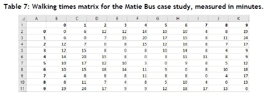
The entry in row t and column j of the walk matrix of Table 7 may be used to determine the cost of the walk arc representing travelling from vertex v_£ to vertex for all the walk arcs of the UTFSP instance. The NSGA II of §4.4 may then be executed to solve the resulting UTFSP instance.