GENERAL ARTICLES

 

Using Monte Carlo simulation to quantify the cost impact of systemic risk factors in a project portfolio: a case study

 

 

F.J. Joubert^{I, *}; M. Snyman^II

^IDepartment of Industrial Engineering, Stellenbosch University, South Africa. https://orcid.org/0000-0002-9871-7442
^IIPrivate. https://orcid.org/0000-0002-8914-3651

 

 

---

ABSTRACT

In terms of project risk management, 'systemic risk' is identified as risks which are artefacts of the environment which a project is executed in, and are related to (i) the project team's actions, (ii) how project controls are managed and interact, and (iii) how the project is planned and executed. This paper proposes a methodology to estimate the cost impact of systemic risk on a portfolio of projects by using risk quantification and Monte Carlo simulation, in the absence of a validated parametric risk model, to estimate the systemic risks in an entire portfolio of projects. The case study simulation results indicate a significant effect of systemic risks on the project portfolio risk profile, where systemic risks increased the P80 value of the contingency requirement by +85.6%. The successful management of systemic risk would contribute to project success by limiting unnecessary waste.

---

OPSOMMING

In terme van projekrisikobestuur word sistemiese risiko' s geïdentifiseer as risiko's wat 'n karakteristiek is van die omgewing waarbinne die projek uitgevoer word. Hierdie risiko' s hou verband met (i) die aksies van die projekbestuurspan, (ii) hoe projekkontroles bestuur word en ineenskakel, en (iii) hoe die projek beplan en uitgevoer word. Hierdie artikel stel n metode voor wat gebruik kan word om die koste-impak van sistemiese risiko's op n projek portefeulje te bepaal waar daar 'n gebrek is aan 'n geldige paremetriese model vir die berekening van sistemiese risiko' s se impak op n hele projekportefeulje. Dit word gedoen deur middel van risiko kwantifisering en Monte Carlo simulasie. Die resultaat toon n noemenswaardige impak van sistemiese risiko' s op die risikoprofiel van die projekportefeulje, waar sistemiese risiko die gebeurlikheidsbegroting met +85.6 % verhoog het. Die suksesvolle bestuur van sistemiese risiko' s kan n noemenswaardige effek op projek sukses uitoefen deur die beperking van onnodige vermorsing.

---

 

 

1 INTRODUCTION

1.1 Simulation developed to support science became science in itself

Nicholas Metropolis coined the term 'Monte Carlo method' in the late 1940s after the first electronic computer-based Monte Carlo method was devised by Stanislaw Ulam while working at Los Alamos National Laboratory (Kamgouroglou, 2020; Metropolis, 1987) as part of the North American nuclear programme. When computers became more widely available from the 1970s onwards, it became possible to apply more sophisticated methods to determining project contingencies (Broadleaf, 2014); and the availability of the first desktop-based Monte Carlo simulation (MCS) software in the 1980s (Hollmann, 2016) opened up a significant new field of project risk management research. Harrison, Lin, Carroll, and Carley (2007) stated that some research on simulation studies started appearing in the 1980s; but it only began to appear regularly in social and management science journals in the 1990s. Harrison et al. (2007, p. 1243) stated that "computer simulation can be a powerful way to do science", and "...computer simulation promises to play a major role in the future..."; they concluded that "computer simulation is now a recognised way of doing science". The published research referred to disciplines related to management, psychology, sociology, economics, and political science. Berends and Romme (1999, p. 576) confirmed Harrison et al.'s view. By 2010, Jahangirian, Eldabi, Nasseer, Stegioulas, and Young (2010b, p. 8) had reviewed several simulation applications published in the peer-reviewed literature on business and manufacturing for the period between 1997 and 2006. They found that MCS was primarily employed in solving numerical problems such as risk management and property valuation.

1.2 What is Monte Carlo simulation, and how is it applied in the project risk management environment?

The Monte Carlo simulation (MCS) method is a computerised mathematical technique that is used in quantitative analysis and decision-making. MCS is used to perform quantitative risk analysis on models approximating a project's behaviour, based on input factors and dependencies, after substituting any factor in a risk model that has inherent uncertainty with a range of values in the form a probability distribution. The simulation calculates the model outcomes repeatedly, each time using a different set of random values that may be represented by different types of input distribution. MCS software then uses up to tens of thousands of iterations to produce a dataset of possible outcome values that may be used to influence project decision-making. Instead of stating, for example, that a project will be completed on 15 May 2026, the software produces a result in which the outcome is linked to a likelihood - something like "There is a 60% likelihood that the project will be completed on 15 May 2026". There are other advantages of MCS, such as that it may be used (i) to conduct a sensitivity analysis, and (ii) to provide a measure of the accuracy of the simulation results. Software is easily available, may be purchased online, and is relatively inexpensive (American Society of Safety Engineers, 2011). What contributes to MSC's popularity is that it can use existing project data and it employs simple statistics Hillson (2009). It is an internationally accepted way of conducting risk assessments, as described in ISO31010 (International Organisation for Standardization, 2019). In the project management discipline, MCS is used to model discrete cost risks and uncertainties related to project schedule delays and project cost. Software packages such as Tamara (Vose Software), Oracle Primavera Risk Analysis (Pertmaster^®), Safran Risk, and Deltek Acumen Risk use MCS to model project schedule risks in terms of both time delay and cost. When modelling cost and schedule in projects, there are two types of methodology (Raydugin, 2018). MCSs form part of the first group, called the computational method, which is based on calculations of expected total cost and schedule outcomes for upcoming projects. The second group, empirical methodologies (i.e., expert opinion, rules of thumb, parametric methods, etc.), are based on data analysis for completed projects with the primary goal of predicting the outcomes of similar projects (Raydugin, 2018). This method was initially used to estimate the effect of risk in projects prior to the increased availability of MCS software (Hollmann, 2016). It is still used, especially in earlier project phases when accurate costing information is not yet available and systemic risks tend to dominate estimate uncertainty.

1.3 Systemic risk

There are various definitions of the term 'systemic risk'. 'System', in turn, is defined as an assembly or combination of elements or parts that together form a complex or unitary whole, and are composed of components, attributes, and relationships (Blanchard & Fabrycky, 1990).

Since the ISO31000:2018 definition of risk provides for objectives to be context-specific, systemic risk is considered in the context of (i) enterprise risk management and (ii) project risk management. Enterprise risk management considers systemic risks as (i) developments that may threaten the stability of the financial system as a whole and consequently that of the broader economy, not just one or two institutions; or (ii) developments in the financial system that may cause the financial system to seize up or break down and so trigger massive damage to the real economy (R. Chapman, 2006). Examples of these risk events are (i) the Great Depression, (ii) the financial crisis of 2007 / 2008, and (iii) the great lockdown of 2020. The objectives that are impacted by these types of risk relate to issues such as economic growth, reducing unemployment, and price stability.

In the project risk management context, these objectives typically relate to meeting the budget and completing the project on time and with acceptable quality while meeting all legal and social obligations. The Association for the Advancement of Cost Engineering International (AACEI) (2016) states that 'project systemic risks' are the opposite of 'project-specific risks', and defines systemic risks as uncertainties (threats or opportunities) that are an artefact of an industry, company, or project system, culture, strategy, complexity, technology, or similar over-arching characteristic. 'Project-specific risks' is used to identify events, actions, and other conditions that are specific to the scope of a project - for example, extreme weather, or abnormal soil and geotechnical conditions - and for which the impacts are more-or-less unique to the project (AACE International, 2016). These types of risk are normally modelled using computational methods such as MCS when the probability of these events occurring is not certain (p<1).

Hollmann (2016) expands on the AACEI definition by defining 'systemic risks' as artefacts of system attributes (the internal project system, its maturity, company culture, and complexity) and the project's interaction with external systems (regional, cultural, political, and regulatory systems). Systemic project risks are regarded as possible additional causes of project-specific cost risks that give rise to nonlinear cost impacts (Raydugin, 2018). The probability that these risks will occur is p=1. C. Chapman and Ward (2011) uses the term 'systemic uncertainty', which involves simple forms of dependence or complex feedback and feed-forward relationships, which include general or systemic responses between sources that have been decomposed.

Therefore, project systemic risks can also be described as the properties or behaviours of a project system whose impact is uncertain owing to the nature of the project system and its interactions with external systems and for which a cumulative impact can be constantly observed (P=1), even if the individual systemic risks occur infrequently (P < 1).

1.4 Parametric modelling of systemic risk

The history and application of these types of model are well described by AACE International (2011), Hollmann (2016), and Raydugin (2018). These models attempt to model a relationship between inputs (e.g., risk factors) and project outcomes (e.g., cost growth) based on the study of empirical data using methods such as multi-variable regression analysis, neural networks, or even trial-and-error. In this context, a typical form of a simple parametric estimating algorithm is as follows:

where:

Constant = Intercept

Coefficient = Regression coefficient for a specific parameter

Parameter = The value of a specific project property metric (AACE International, 2011)

The main advantages of using parametric estimating for risk analysis and contingency determination are that (i) it is empirical in nature (i.e., it is based on actual measured experience), and (ii) it is quick and simple. Disadvantages include that, because these empirical methods are based on regression analysis, which requires predictable relationships between inputs and outputs, the method is typically limited in application to the estimating of the overall project contingency required for selected risk types, and that the contribution of individual parameters cannot be isolated. Raydugin (2018) presented a method that uses MCS to model systemic risks in single projects, specifically in the context of weak project teams. The risk-factoring method described by Broadleaf (2014) can also be used to model systemic risk in single projects.

The authors of the current study, and Boyle (2020) noted that, in the construction industry, systemic risks are typically not considered on their own as part of a quantitative risk analysis. In the rare cases when they are raised, the argument tends to be that they are included in the quantified uncertainty ranges, or that they are less significant than the project- specific risks. Thus any "allowance" for systemic risks disappears into the model and can't be observed in the outputs. The results of this research indicate that systemic risks could have a significant effect on project performance and should be addressed as a separate feature of QRA's. The challenge with this is that there is no accepted method for consistent identification or quantification of systemic risks in the absence of a validated parametric model or sufficient time to develop one if adequate historical data is available.

1.5 Simulating risks in a portfolio of projects

The methods described earlier in this paper all deal with the modelling of risks in a single project. A project hierarchy is described in PMBoK™ (Project Management Institute, 2013), in which projects roll up into programmes, and programmes roll up into portfolios. C. Chapman and Ward (2011) and Hillson (2009)shares this view. Given their nature, portfolios and programmes are more complex systems to manage than single projects. When doing a literature search for articles related to simulation models and the quantification of risks in a project portfolio, limited information could be found. The manufacturers of simulation software such as Palisade Corporation (2014) and (Vose, 2008) define 'portfolio' in terms of finding an optimal investment portfolio, and do not specifically discuss methods that may be employed in modelling risks in an entire capital project portfolio. Schedule simulation on single projects is covered by various authors, such as AACE International (2008), Elshaer (2013), and Trietsch and Baker(2012). These, however, tend to focus on single projects and not the simulation of a portfolio of projects. The search for multi-project and programme risk management and simulation methods also presented limited results. Lytvyn and Rishnyak (2014) presented a decision-making algorithm that can be employed when a project is influenced by a multi-project environment. The current study uses methods described by Joubert and Pretorius (2017) to model the extent of systemic risks in a portfolio of capital projects.

1.6 Data used

The research data was collected over four years while the author was employed by a South African freight logistics company (FLC) that also had a capital projects division. The projects' scope primarily included rail and port infrastructure capital projects. The organisation used a quantitative risk assessment model using @Risk software to create risk registers for a portfolio of 106 projects. These projects were distributed over the concept, project development, and project execution phases of the project lifecycle.

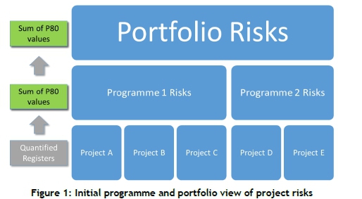
To analyse risks on a portfolio basis, the simulation results of the individual project risk registers were uploaded into a Risk information management system. The way in which portfolio-level project risk information was extracted and aggregated by the FLC from this system was (i) to count the frequency of the individual risks and (ii) to aggregate the P80 values of the individual risks, as shown in Figure 1. If the risk 'inclement weather' appeared 25 times, the P80 values of each of these risks were simply summed. The FLC knew that this method was mathematically incorrect, but at least it indicated which risks appeared throughout the project portfolio, and which aggregate risk had the most significant possible consequences.

 

 

1.7 Research objective

To understand the role of systemic risks in a project portfolio, a more scientific method had to be developed to provide insight into the questions below:

1. How can the identified systemic risks be quantified?

2. What is the extent of systemic project risks in the portfolio of projects?

3. What type or category of systemic risk caused the most uncertainty in the project portfolio?

4. Which individual systemic risks caused the most uncertainty in the portfolio of projects?

5. In which type of project (scope-related) is the most significant amount of systemic risk found?

A more thorough understanding of systemic risk in a portfolio of projects is important. Since the risks are systemic by nature, the treatment plans for systemic risks usually rely on elements that cannot be treated successfully on a project or programme level. An example of this would be the risk 'approval delays' in an organisation with a lack of commitment to starting project execution. A typical example of this would be delayed project approvals owing to a lack of stakeholder commitment. The consequence of this would not only be the delayed implementation of project benefits, but also the effect of escalation on the project cost. From a project resource perspective, project teams might be wasting time by attempting to treat systemic risks - or, more likely, risks with strong systemic causes - that are beyond their ability and mandate to treat. Should the systemic risks be identified, they would be best treated at their origin, not where their consequences manifest. Systemic risks tend to be associated with business processes, including project management processes, used by or interacting with a project. By treating systemic risks, multiple current and future projects would benefit.

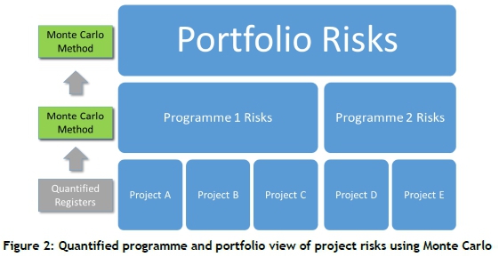
This paper therefore proposes a methodology that uses a set of individually quantified risk registers, MCS (@Risk software), risk names, and systemic risk types and sub-types to understand the extent of the impact of systemic risks on a portfolio of projects, as shown in Figure 2.

 

 

2 METHOD

The basic principle of this methodology is to be able to compare different sets of simulation results with one another to determine the effect of one type of systemic risk on the entire project portfolio. The process has the following steps:

1. Classify all of the risks in the project portfolio as being either (i) project-specific or (ii) systemic.

2. Create a project portfolio simulation dataset that includes all of the project-specific and systemic risks.

3. Create a simulation dataset called 'Project-specific risks only' in which all of the project-specific risks are removed from the simulation results.

4. Compare the descriptive statistics (mean, percentiles) of the project-specific risks with only the project portfolio simulation dataset to determine the effect of the systemic risks on the project portfolio.

The rest of this section describes how the model was compiled.

2.1 Consolidate risk registers and review risk names

The first step was to consolidate the existing risk registers into a single MS Excel spreadsheet to accommodate a concurrent MCS. This spreadsheet was based on the existing project risk register template. The initial portfolio included 106 risk registers. Of these, 86 were suitably complete and could be copied into a complete risk register (CRR) that contained 329 different risk names, representing 1063 individual risks.

The next step was to review all of the risk names to ensure a consistent use of the naming conventions. Risk names such as 'inclement weather' and 'bad weather' were consolidated into 'inclement weather', and risk names such as ' industrial action', ' labour unrest', and ' strikes' were merged into ' industrial action'. At the end of this exercise the 329 risk names had been reduced to 166.

2.2 Categorise projects

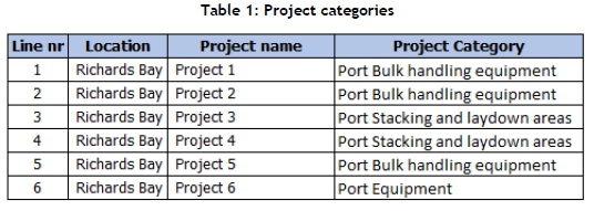
Projects have many characteristics and attributes that can be used as criteria to categorise them. Crawford et al. (Crawford, Hobbs, & Turner, 2004) described various ways in which project can be classified, including (i) scope, (ii) stage of life-cycle, (iii) timing, (iv) risk, and (v) complexity. From this list, scope (the project category in Table 1) was selected, since FLC customers have specific businesses objectives that in turn influence the different varieties of project that they might require. Each of the different projects was therefore assigned to a list of 15 project categories. A sample of this classification is given in Table 1, where 'project types' refers to 'project categories'. Using the PMBoK™ (Project Management Institute, 2013) project hierarchy, the list of projects assigned to a project type would make up a programme, and all of the programmes would constitute the portfolio.

 

 

2.3 Categorise systemic risks and link the risks to the combined risk register

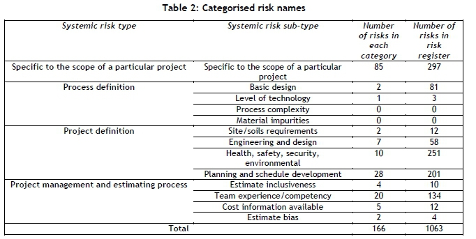
A new sheet, 'Risk names', was created. This was then populated with the various risk names, and each of the projects was classified. Risks that were project-specific, not systemic, were classified as 'project-specific to the scope of a particular project'. The remainder of the risks were classified according to the typical main and sub-type of systemic risks, as listed in Table 2 and by AACEI in RP 42R-08 (AACE International, 2011). As a rule, for each risk name, the underlying project level risks were reviewed to help determine whether the underlying risks had significant systemic causes that originated inside the project system boundary and that were relevant to the portfolio of projects. For the purpose of the classification, the project system boundary included all of the parties contracted to execute the project, as well as the SOE's business processes and systems that were used by the projects. In cases where the classification structure could not easily classify all of the risks, the priority was to ensure that the risk was at least classified correctly as being either systemic or project-specific. These classifications were then linked to the CRR to be used in the simulation. Table 2 lists these categories, the number of risks categorised into each category, and the number of risks in the CRR for each of the categories.

2.4 Existing risk quantification model

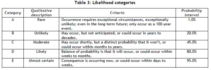
The risk quantification model allowed for single- and multiple-occurrence risks. The table below describes the probability values used for single occurrence risks. These values were selected from the likelihood ranges prescribed by the FLC's enterprise risk management policy, since @Risk requires discrete values to simulate likelihood.

Likelihood scales, as presented in Table 3, represent the probability part of the probability-impact grids (PIGs) described by Hillson (2009, p. 38) and Cooper et al. (2005, p. 53). There are various criticisms of these matrices, including their focus on threats and the exclusion of opportunities, as well as their inability to support complex decision-making (2009, p. 39), (2008), (2011, p. 49). A further inadequacy is that they do not provide for multiple occurrence risks, and do not assess risk urgency. However, the matrices were what were used in the FLC's risk register template (RRT).

The likelihood of single occurrence risks was modelled using a binomial distribution. This is a discrete distribution that returns integer values greater than or equal to zero (Palisade Corporation, 2014). However, there are risks that might occur multiple times in a single project, such as inclement weather, industrial action, and late material deliveries. A Poisson distribution was used to model the frequency of these risks. This discrete distribution returns only integer values greater than or equal to zero (Palisade Corporation, 2014).

Estimating consequence

Risk consequence was modelled in respect of the financial impact on the project, using the following formula:

where:

This application can be described using the following example. A project has two contractors, Contractor A (weekly average rate of R20 000) and Contractor B (weekly average rate of R5 000). During the risk workshop it is established that, should a specific risk realise, Contractor A will have a 10% loss and Contractor B a 100% loss. The weekly weighted average cost would therefore be as follows:

To ensure that sampling takes place at the tail end of more uncertain risks, two different distributions that accentuate long tails were used to simulate three-point estimates. By modelling the minimum value as a P5 and the maximum as a P95, these distributions compensate for quantification bias by extending the distribution beyond the estimated values in the same way as a trigen distribution does.

when

Taking the above, the overall logic used in creating the simulation results appears in Figure 3.

It should be noted that the choice of distributions and the assignment of their parameters were done to attempt to answer the research questions that didn't include validation of the model against actual data.

2.5 Create reports

The next step was to generate reports. The MS Excel name manager tool was used to identify the columns in the CRR that were going be used in the reports. This step significantly simplified the creation and understanding of the formulas, and the following named ranges were created: (i) Project_Category, (ii) Risk_Name, (iii) Simulation_Result, (iv) Risk_Systemic_Type, and (v) Risk_Systemic_Type_Sub. This method allowed tornado graphs to be created for specific data input combinations. These graphs present sensitivity analysis results that display a ranking of the input distributions that impact the simulation results. The longer the bars on the graph, the more the simulation inputs are correlated with the outputs (Palisade Corporation, 2014). The following syntax was used:

This may be interpreted as: Produce a simulation output where the project category equals 'rail power supply' and the systemic risk type equals 'engineering and design'.

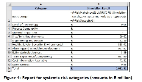
In some instances, the use of =RiskOutput() did not produce the intended result, as the tornado graphs treat likelihood and consequence of a single risk as separate inputs. In these cases, the =RiskMakeInput() function was used, since it specifies that the calculated value for a formula is treated as a simulation input, in the same way as a distribution function. The effect is that the values of the variables in the preceding cells feeding into the =RiskMakeInput() function are used in the calculation, but the variables in the preceding cells do not appear in a tornado diagram linked to the =RiskMakeInput() function cell. The next step was to generate reports using the above principles. Figure 4 shows the use of =SumIfs(), =MakeRiskInput(), and =RiskMakeOutput() in generating output distributions for the systemic risk categories.

 

 

3 FINDINGS

The findings for the simulation results below are discussed, and relate to research objectives 2 to 5 as discussed in paragraph 1.7:

• Extent of systemic project risks' impact on the project portfolio.

• Systemic risk categories causing the most uncertainty in the project portfolio.

• Individual systemic risks causing the most uncertainty in the project portfolio.

• Project type (scope-related) with the most significant risk.

3.1 Extent of systemic project risks' impact on the project portfolio

The simulation model was run for 10 000 iterations, and the results indicated that systemic risks have a significant impact on the project portfolio. When the systemic risks are included in the project portfolio, the mean of the entire project portfolio contingency requirement increases from R2 456.0 million to R4 557.8 million (+85.6%) (Figure 5). The green graph (entire portfolio) presents the sum of the simulation results of the blue graph (systemic risks) and the red line (project-specific risks). This result is impacted by the choice of impact distributions and the assignment of parameters. It can be reasonably assumed, however, that using validated distributions will not indicate that the systemic risks' effect on portfolio level is negligible.

This can be measured in two ways: by (i) using a tornado graph, or (ii) comparing the mean or P80 values of the individual systemic risk categories.

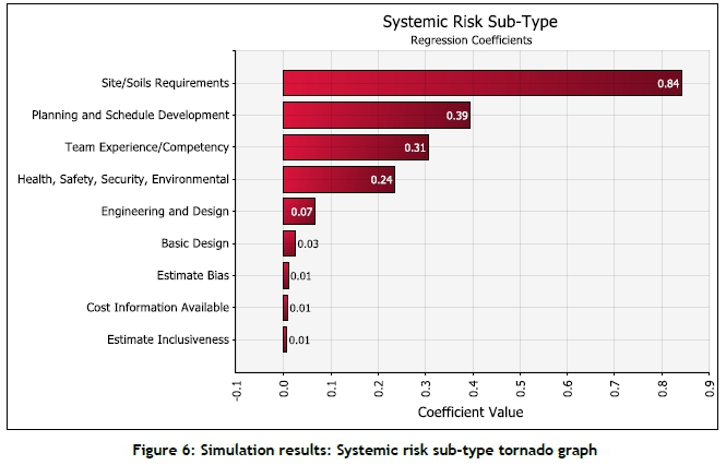
The tornado graph of the systemic risks in Figure 6 identifies site/soils requirements as the top driver, while -when comparing the means in Table 4 - the planning and schedule development category resulted in the highest mean per risk category. The reader will observe that there are some similarities between the sequence of the risk categories in Figure 6 and Table 4, but that there are also several significant differences in the ranking sequence for the same risk category between Figure 6 and Table 4.

When reviewing the CRR, it was found that the category site/soils requirements contained risks related to site access. This makes sense in the context of the FLC, in that there is a recurring theme of the organisation's operating divisions not handing over project sites to the capital projects divisions on time. Regression coefficients are presented in @Risk using tornado diagrams, which measure the tendency of the value of the output cell used to vary, depending on the value of the input variables. The percentage variation in the inputs, risks, output results, and discrete values, such as an estimate value or schedule duration, has a significant effect on the output results of a model and therefore on the regression coefficients displayed in tornado diagrams. Thus it is important to understand the features of the software and of the model used to avoid a misinterpretation of the tornado results. This is especially important when a risk model is combined with a schedule and a CAPEX QRA model, as this can result in even more misleading results.

3.2 Systemic risk categories causing the most uncertainty in the project portfolio

When reviewing the mean of the various categories, it was found that planning and schedule development category had the highest mean of all the categories. This category included risks such as (i) approval delays, (ii) contracting strategy, (iii) contractor quality, (iv) operational readiness, and (v) unavailable equipment.

Because of the definition of the mean's calculation, the mean does not indicate the potential effect of the extreme values of the input variables, and so it should be used with caution if some of the output results being compared produce values across a wide range. In such a case, using an additional comparison of P80, or possibly even P90, values on the high side and P10 or P20 on the low side would be useful to guide decisions on which items to prioritise for action.

3.3 Individual systemic risks causing the most uncertainty in the project portfolio

For this section, the reader needs to be reminded that the systemic risks discussed in this section refer to a type of risk, and that the model would typically include a number of the same systemic risks across the portfolio, but only one record per project.

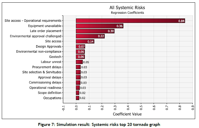
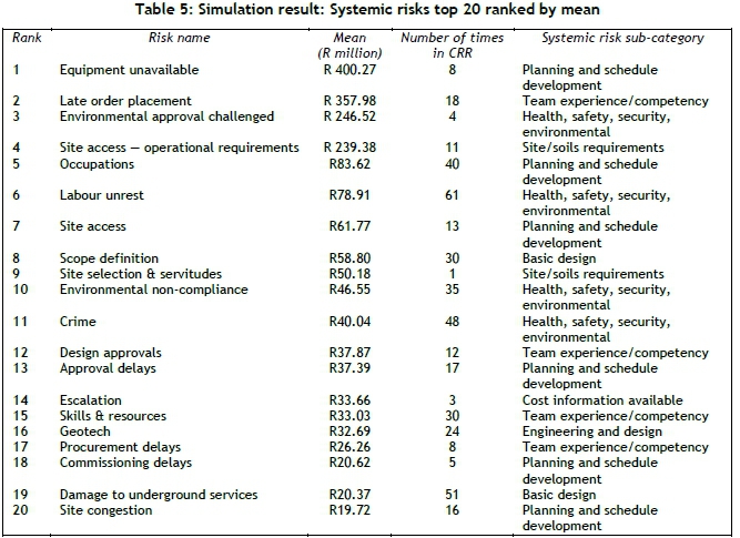
The results of the individual systemic risks are also presented by way of a tornado graph and a table containing the category means. The tornado graph in Figure 7 shows that the most important systemic risk is the site access - operational requirements risk. This risk belongs to the site/soils requirements category, which was the top driver in Figure 6's regression tornado. The other risks in the site/soils requirements category appear much lower down in this tornado. When comparing Figure 7 with Table 5's comparison of the individual risks' ean value, there are some noticeable differences in the sequences. These are largely caused by the same mechanisms that were explained in the discussion of the category level results.

The next table lists the top 20 systemic risks, ranked according to the mean of the related risk's output distributions.

3.4 Project type (scope-related) with the most significant risk

It would also be important to review the results indicating in which project category (as defined earlier) systemic risk would be the most prevalent. As before, the results are presented in both tornado graphs and a table of the means, as shown in Figure 8.

Table 6 lists all of the project categories, ranked according to the mean of the related risk's output distributions.

 

4 DISCUSSION

4.1 Simulation results and future research

The simulation results model quantified the importance of identifying and treating systemic risks on a programme and portfolio level, since it indicated that the system risks more than doubled the mean value of the project-specific risks simulation. It contributes to the body of knowledge because it shows how readily accessible simulation packages (such as @Risk) can be used to determine the effect of systemic risks in a portfolio of capital projects.

As the data used for the models discussed in this paper was based on risk registers, it contained predictions by the assessment team. The application of this approach could be expanded to enable the reliable identification of systemic risk factors, and to establish guidelines for these factors' uncertainty ranges and a method for parameter verification if sufficient suitable data is available. The authors have started to explore the following next steps:

1. Establish a method to extract actual systemic risk data from the project performance data of completed projects, and establish whether the actual impacts of systemic risks on completed projects are as important as indicated in this research.

2. Explore the effect and importance of the individual business process controls associated with all of the systemic risks in a portfolio or similar projects - for example, do they sum or accentuate each other?

3. Develop a suitable systemic risk categorisation system that allows categorisation of the systemic risks and their underlying variables.

4. Develop a verifiable set of quantified risk factors that can be applied in quantitative project risk analysis, thereby improving the credibility of the results. Systemic risks are very similar to the concept of risk factors used in cost and schedule simulation software packages when the issue of risk factor quantification is a challenge.

4.2 Lessons learnt

1. During the building of the model, some lessons were noted that could have an impact on future research and on the practical implementation of the proposed methodology. The first was that the classification of risks into the various systemic risk categories proved to be problematic, and resulted in extensive discussions about how the risks were classified. It is recommended that the classification of this be done in a workshop environment attended by suitable subject-matter experts. The definition of systemic risks needs to be clear, and the boundaries of the system in which they may arise need to be clearly defined. It is also recommended that, after the risks have been classified, the various groups of classified risks should be reviewed to ensure that there is internal consistency in them.

2. In the discussions about systemic risk classification, the following properties were noted that made classification particularly challenging: (i) project-specific risks can turn into systemic risks over time; (ii) some risks display both systemic and project-specific properties at the same time, such as a contractor's poor procurement process for critical equipment; (iii) project-specific risks can lead to systemic risks - for example, in an attempt to manage a project-specific risk, cumbersome processes could be imposed; and (iv) project-specific risks and their causes can be used to predict where there might be systemic risks.

3. The systemic risk classification system used was also problematic in that it was focused on systemic risks found in the design and construction of process plants. This was evident in the categories process complexity and material impurities not having any risks assigned to them. A structure that provided for port and rail construction projects could have been more useful, and so establishing such a structure is a topic for future research.

4. It is also important to note that there was value in reviewing the simulation results using both tornado graphs and tables to present the means of the various simulation results, as they show the simulation results in respect of both variability and order of magnitude. The latter can be used to present the business case for further analysis of the identified focus areas to enable treatment planning or, if possible, to implement the required treatment plans already identified.

5. The method that was applied when risks in a portfolio were classified as either systemic or project-specific and then included or excluded from the simulation results to determine the effect of systemic risks on the portfolio can, of course, also be applied to individual projects. This in itself is useful in providing a potential treatment plan cost justification for systemic risks on a project level.

4.3 Limitations

Some limitations were also encountered during the research. Some simulation models may be too complex; and so Axelrod (1997), Vose (2008, p. 7), and Marsh (2013) advocate the use of simple models, as it is then easier to gain insight into causal relationships. The model presented in this paper is relatively simple, as it circumvents long, complex equations, avoids using any macros, and is contained in a single worksheet. Simulation models that are not presented in sufficient detail may be difficult to verify and validate independently, thus reducing the reliability of the research results (Harrison, Lin, Carroll, & Carley, 2007, p. 124). The simple model presented in this paper, together with the way in which the model has been described, should overcome this shortcoming.

Some issues with independent verification might also be encountered. By their nature, simulation experiments are artificial, since they are based on computer models in which the simulation data is computer-programme generated (Harrison, Lin, Carroll, & Carley, 2007, p. 1241). The data used in this research was based on data supplied by subject-matter experts. Eppen et al. (1988, p. 2) call models like this a "selective abstraction of reality". This in turn raises the question of how the simulation model is aligned to real-world behaviour. This may be remedied by comparing the simulation results with empirical work, and by basing some of the simulation model's parts on empirical work. Model validation is therefore included as a step in the development of quantitative models (2005, p. 259), (2008, p. 5). An example in this paper is the validation of criteria used to select which risks to model with long tails and the choice of PERT and lognormal distributions for the selected risks; and the assignment of these distributions' parameters could well have resulted in somewhat different results if different choices had been made. Further research on these aspects would be advisable prior to applying them in practice.

Both Vose (2008, p. 5) and Palisade Corporation (2014) emphasised the importance of using correlation in simulation models. The simulation model presented in this paper contains data from 86 different projects with 1063 individual risks. This would require a 1063 by 1063 correlation matrix to be part of the model. Given the dynamic and complex nature of such a matrix, it had to be assumed that all of the risks were independent, which made the requirement of a correlation matrix redundant.

Broadleaf (2014) stated that there is evidence that, when considering a large number of items, realistic correlation modelling is rarely practised. Since project contingency was only simulated in the risk registers, and no integration between the risk register, the cost estimate and the schedule took place, no comment can be made about the impact of systemic risks on the project schedules that form part of this project portfolio. The main reason for this is that the authors did not have access to the schedules of the individual projects, and also that they were not aware of any schedule simulation software that would be able to run such a concurrent schedule simulation and the required data analysis for this methodology.

 

5 CONCLUSION

This research would not have been possible without the advances in ICT during the last 40 years, which allowed the development of desktop MCS cost-simulation software that can be used to quantify project cost and schedule contingencies. This paper presents a novel methodology that could be used (i) to estimate the impact of systemic risks on a portfolio of capital projects; (ii) to determine the relative importance of the specific systemic risks and their categories; and (iii) identify a ranked list of 20 systemic risks that could be used as a checklist for similar projects or portfolios. The inclusion of systemic risks in the existing project-specific risk dataset had a significant impact, since it increased the mean of the project contingency dataset by 85.6%. This result confirms the importance of identifying and implementing suitable treatment plans for systemic risks as part of a project management system quality improvement drive. Although some limitations are mentioned, the method is still valid for identifying the most important systemic risks for further analysis before suitable treatment plans are implemented.

 

REFERENCES

[1] Kamgouroglou, G. 2020. Metropolis, Nicholas Constantine (1915-1999). Available from: http://scienceworld.wolfram.com/biography/Metropolis.html [Accessed 04 05 2020].         [ Links ]

[2] Metropolis, N. 1987. The beginning of the Monte Carlo method. Special edition. Los Alamos Science, Los Alamos.         [ Links ]

[3] Broadleaf. 2014. Weaknesses in common project cost risk modelling methods. Cammeray: Broadleaf Capital International.         [ Links ]

[4] Hollmann, J. 2016. Project risk quantification. Gainesville, Florida: Probalistic Publishing.         [ Links ]

[5] Harrison, R., Lin, Z., Carroll, G., & Carley, K. (2007).. Simulation modelling in organizational and management research. Academy of Management Review, 32(4) pp. 1229-1245.         [ Links ]

[6] Berends, P. and Romme, G. 1999. Simulation as a research tool in management studies. European Management Journal, 17(6) pp. 576-583.         [ Links ]

[7] Jahangirian, M., Eldabi, T., Naseer, A., Stergioulas, L., & Young, T. 2010. Simulation in manufacturing and business. European Journal of Operational Research, 203(1) pp. 1-13.         [ Links ]

[8] American Society of Safety Engineers. 2011. ANSI/ASSE/ISO Guide 73 (Z690.1-3011) Vocabulary for risk management. Des Plaines, Illinois: American Society of Safety Engineers.         [ Links ]

[9] Hillson, D. 2009. Managing risk in projects. Farnham: Gower Publishing.         [ Links ]

[10] International Organization for Standardization. 2019. ISO31010:2019 Risk management - Risk assessment techniques. Geneva: International Organization for Standardization.         [ Links ]

[11] Raydugin, Y. 2018. Non-linear probabilistic (Monte Carlo) modeling of systemic risks. AACE International Conference & Expo.24-27 June 2018, San Diego, CA.         [ Links ]

[12] International Organization for Standardization. 2018. ISO31000:2018 Risk management guidelines. Geneva: International Organization for Standardization.         [ Links ]

[13] Blanchard, B. and Fabrycky, W. 1990. Systems engineering and analysis. Englewood Cliffs, New Jersey: Prentice Hall.         [ Links ]

[14] Chapman, R. 2006. Simple tools and techniques for enterprise risk management. Chichester: John Wiley & Sons.         [ Links ]

[15] AACE International. 2016. 10S-90 Cost engineering terminology, Morgantown, WV.         [ Links ]

[16] Chapman, C. and S. Ward. 2011. How to manage project opportunity and risk. Chichester: John Wiley & Sons.         [ Links ]

[17] AACE International. 2011. 42R-08 Risk analysis and contingency determination using parametric estimating. AACE International, Morgantown, WV.         [ Links ]

[18] Boyle, J. 2020. Comments on systemic risks in construction projects, M. Snyman, Editor.         [ Links ]

[19] Project Management Institute. 2013. A guide to the project management body of knowledge (PMBOK). 5^th ed pp. 316. Newton Square, Pennsylvania pp. 316.         [ Links ]

[20] Palisade Corporation. 2014. @Risk help file.         [ Links ]

[21] Vose, D. 2008. Risk analysis: A quantitative guide. Chichester: John Wiley & Sons.         [ Links ]

[22] AACE International. 2008. 65R-11 Integrated cost and schedule risk analysis and contingency determination using expected value, Morgantown, WV.         [ Links ]

[23] Elshaer, R. 2013. Impact of sensitivity information on the prediction of project's duration using earned schedule method. International Journal of Project Management, 31(4) pp. 579-588.         [ Links ]

[24] Trietsch, D. and Baker, K. 2012. PERT 21: Fitting PERT/PM for use in the 21st century. International Journal of Project Management, 30(4) pp. 490-502.         [ Links ]

[25] Lytsyn, V. and Rishnyak, I. 2014. Modeling and evaluation of project risks in multi-project environment. Informatyka, Automatyka, Pomiary w Gospodarce i Ochronie Srodowiska, 4(2) pp. 34-36.         [ Links ]

[26] Joubert, F. and Pretorius, L. 2017. Using risk simulation to reduce the capital cost requirement for a programme of capital projects. Business, Management and Education, 15(1) pp. 1-13.         [ Links ]

[27] Crawford, L., Hobbs, J. and Turner, R. 2004. Project categorization systems and their use in organisations: An empirical study. PMI Research Conference, Project Management Institute, London.         [ Links ]

[28] Cooper, D., Grey, S., Raymon, G., & Walker, P. (2014). Project risk management guidelines. Chichester: John Wiley & Sons.         [ Links ]

[29] Cox, L. 2008. What's wrong with risk matrices? Risk Analysis, 28(2) pp. 497-512.         [ Links ]

[30] Axelrod, R. 1997. The complexity of cooperation: Agnet-based models of competition and collaboration. Princeton, New York: Princeton University Press.         [ Links ]

[31] Marsh, C. 2013. Business and financial models. London: Kogan Page.         [ Links ]

[32] Eppen, G., Gould, F. and Schmidt, C. 1988. Quantitative concepts for management: Decision making without algorithms. Engelwood Cliffs, New Jersey: Prentice-Hall.         [ Links ]

 

 

Submitted by authors 12 Apr 2021
Accepted for publication 4 Oct 2021
Available online 14 Dec 2021

 

 

* Corresponding author: kwanto.risk@gmail.com