SPECIAL EDITION

 

Using machine learning to predict the next purchase date for an individual retail customer

 

 

M. Droomer^*; J. Bekker

Department of Industrial Engineering, University of Stellenbosch, South Africa

 

 

---

ABSTRACT

Targeted marketing has become more popular over the last few years, and knowing when a customer will require a product can be of enormous value to a company. However, predicting this is a difficult task. This paper reports on a study that investigates predicting when a customer will buy fast-moving retail products, by using machine learning techniques. This is done by analysing the purchase history of a customer at participating retailers. These predictions will be used to personalise discount offers to customers when they are about to purchase items. Such offers will be delivered on the mobile devices of participating customers and, ultimately, physical, general paper-based marketing will be reduced.

---

OPSOMMING

Teiken-bemarking het in die laaste jare gewild geword en dit kan baie waardevol wees vir 'n onderneming om te weet wanneer 'n kliënt 'n produk benodig. Hierdie soort voorspelling is egter baie moeilik, en hierdie artikel beskryf 'n studie wat met behulp van masjienleer-tegnieke ondersoek het wanneer n kliënt vinnig-bewegende kleinhandel produkte sal koop. Dit is gedoen deur die koopgeskiedenis van n kliënt by deelnemende kleinhandelaars te ontleed. Hierdie voorspellings sal gebruik word om persoonlike afslagaanbiedinge aan kliënte te maak wanneer hulle produkte wil koop. Hierdie aanbiedinge sal op deelnemende kliënte se mobiele toestelle aangebied word en uiteindelik sal veralgemeende, papier-gebaseerde bemarking verminder word.

---

 

 

1 INTRODUCTION

We live in a world that is rapidly changing when it comes to technology. The use of paper is becoming redundant; for example, more forms are being filled in online, newspapers can be read online, and assignments can be handed in electronically. Signing up for a new mobile application is the new norm, including applications to track sleeping patterns, or fitness levels, or even just an application to play a game. Gathering a customer's information becomes easier as companies have loyalty programmes that track their purchasing behaviour. We live in an era when search engines suggest your next word, online shopping is no longer scary, and people order a ride using an application. The fact is that technology is evolving, and gathering information from customers is becoming easier. Given these changes, the questions, however, are: 'How do companies use this information to gain a competitive advantage?'; 'Do they use this information to benefit the customer?'; 'How can a company use customer information to give everyone a different experience?'.

Marketing has shifted from being product-oriented to being customer-oriented, and in this information-rich era customer behaviour can help marketing managers to choose the most effective marketing strategy for their customers [1]. If a company knows exactly what a customer wants to purchase at a specific time, the company can market according to the customer's needs and potentially gain a competitive advantage. Predicting a customer's purchasing behaviour opens doors for companies to market to a specific individual at the right time. This will have a different impact on a customer than that of the traditional pamphlet in the printed newspaper.

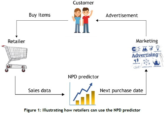
A study was conducted to investigate whether or not machine learning can be used to predict when an individual will purchase fast-moving retail products, based on their past purchasing behaviour. Figure 1 illustrates how a retailer can use the predictor to market to the customer. The customer buys items from a retail store. The retail store captures the customer's purchase history, and provides the sales data to the proposed next purchase date (NPD) predictor. The NPD predictor uses machine learning techniques on the given sales data to determine when the customer will purchase a certain product again. This information is then provided to the marketing team, who can use this information to advertise to an individual at the appropriate time.

 

 

2 LITERATURE REVIEW

Several studies have been done to predict what customers will buy, notably in the fast-moving consumer goods sector. These studies include market basket analysis, predicting customer shopping lists, and predicting a next purchase date to cross- and up-sell items to customers. The main idea of market basket analysis is to know which products customers buy at the same time, to improve marketing. Say, for example, a customer often buys product A with product B, then a discount can be offered on the combination or on one of the products, provided the other product is bought. It is used to increase sales and maintain inventory by focusing on point-of-sale transaction data [2]. It is also used by retailers to determine the store layout, and to ensure that products that are frequently purchased together are located near each other in the store [3].

A different study related to customer purchasing behaviour by Cumby, Fano, Ghani, and Krema [4] predicted a shopping list for an individual customer. This list was displayed to the customer when entering the store to remind them to buy certain products while in the store. The business case for this study was that if a realistic shopping list could be predicted for a customer, the customer would be reminded of items that would otherwise be forgotten. This means that the suggestions are translated into recovered revenue for the store that might otherwise be transferred to a competitor, or even foregone, as the customer would only buy the item when they visited the store again [5].

A study by Els [6] included the development of a personalised discount offer system. The system proposes a personalised discount offer to a customer when they visit the store. These offers are only valid for a specific customer for a specific period of time. In this system, the customer is subject to cross- and up-selling. Say, for instance, a customer enters the store and wants to buy shampoo. Cross-selling an item means that the system suggests conditioner to the customer, to try to sell items that are frequently bought together. Up-selling, on the other hand, would be if the same customer wanting shampoo gets an offer for a different shampoo that is in a higher price range than the shampoo that the customer wanted to buy.

This creates opportunities for alternative revenue streams. Els [6] also attempted, using analytical techniques, to predict when a customer would buy certain products.

This paper seeks improved methods to predict when a customer will buy products. This can be used by retailers to gain competitive advantage. Marketing managers can determine how they want to market to an individual, given that they know when that individual needs specific products. This shifts the marketing strategy from being product-oriented to being customer-oriented.

2.1 Machine learning techniques used

This paper focuses on four techniques to develop the NPD predictor. Two of these techniques - recurrent neural networks (RNN) and linear regression - will look only at the sequence of one user-product pair, while the other two techniques - artificial neural networks (NN) and extreme gradient boosting - will look at the bigger picture by using all the data from all the user-product pairs. A brief explanation of how these techniques work will be given next.

2.1.1 Artificial neural network (NN)

An artificial neural network, referred to as a 'neural network' (NN) in this paper, is a set of connected neurons that are organised in layers. As seen in Figure 2, there are three types of layer:

 

 

Input layer - this layer brings the data into the system to be processed further by the subsequent layers.

Hidden layer(s) - this layer(s) lies between the input and output layers, where artificial neurons take a set of inputs that are weighted, and produce an output through an activation function.

Output layer - this layer is the last layer of neurons (it could be one or more neurons), which produces a given output for the system.

2.1.2 Recurrent neural network (RNN)

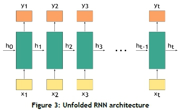
RNNs are neural networks that are good at modelling sequential data [7]. This technique is used for sequential signals such as speech recognition, stock prediction, and language translation. As with a feed forward neural network, RNNs also have an input layer, a hidden layer, and an output layer. However, an extra loop is added that can pass information forward. RNNs use the output of the previous step as the input for the current step. Figure 3 shows the architecture of an RNN, with x₁being the input for the first step, h₀being the hidden value for the first step (which must be initialised), and y₁being the output variable for the first layer. It is called recurrent, as h₁is then passed on and contains information on the first iteration. This is one representation of RNNs, but they can also have multiple inputs with only one output, or one input with multiple outputs.

 

 

2.1.3 Linear regression

Linear regression is a statistical approach to modelling the relationship between a dependent variable and one or more independent variables. For linear regression, a line is fitted through the data according to a specific mathematical criterion. This line can, for example, be fitted to minimise the sum of squared distances between the data and the line. This allows an estimation of the dependent variables [8]. This technique is widely used, mostly for prediction or forecasting.

Linear regression is commonly modelled as Y_t = f(X_t,B) + e_;, where Y_trepresents the dependent variable, X_trepresents the independent variable, B represents an unknown parameter, and e_trepresents the error term. The goal is then to estimate the function f(X_t,B) that best fits the data. The parameter B is estimated by using various tools provided by regression analysis, such as the least squares method, which finds the value of B that minimises the squared error between the line and the data. After this value is estimated, the data can then be fitted for prediction.

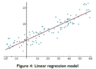
Figure 4 shows the modelling of n data points. There is a single independent variable and two unknown parameters. The line is represented by the equation y_l = B₀ + B₁x_l + e_uwhere i = 1, ...,n. So, given a random sample from the population, the estimated population parameters are obtained, and the sample linear regression model can be represented as y_t = B₀ +B_iX_i. The error e_tis the difference between the dependent value and the predicted dependent value. Minimisation of an error function is used to yield the parameter estimators.

 

 

2.1.4 Extreme gradient boosting (XGBoost)

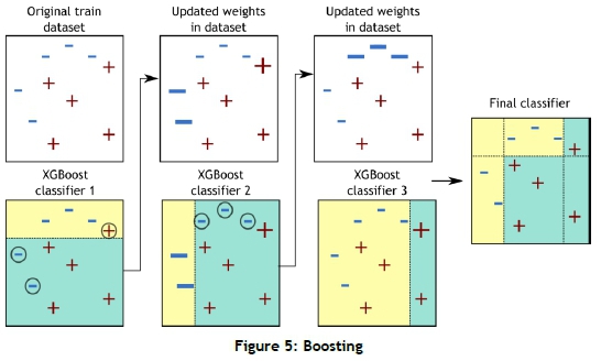
Extreme gradient boosting was developed on the framework of gradient boosting [9]. Boosting, also known as the 'sequential ensemble method', creates a sequence of models in which the models attempt to correct the mistakes that were made in the previous model in the sequence. The first model is built based on the training data, then the second model attempts to improve on the first model, after which the third model attempts to improve on the second model, and so on.

Figure 5 shows that the original data is passed to the first classifier. The yellow area represents the predicted blue hyphen, and the blue area represents the predicted red cross. Thus, for this first attempt, the classifier misclassified the three circled instances. After this, the weights of these incorrectly classified instances are adjusted and sent to the second classifier. The second classifier then correctly predicts the three instances incorrectly predicted by the first classifier, but incorrectly predicts three different instances. This process is then repeated until the specified number of iterations is reached, or a certain threshold is reached by the classifier.

 

 

Gradient boosting uses an approach where a new model is created that predicts residuals (errors) of the prior models that, when added together, make the final prediction. Gradient boosting uses gradient descent to minimise the loss function (the difference between the predicted value and the actual value).

The objective function of the XGBoost model can be calculated by adding the loss function with a regularisation component. This means that the loss function has predictive power, and the regularisation term controls the simplicity and the overfitting of the model.

XGBoost can be used for both regression and classification problems, with a loss function such as root mean squared error for regression versus a loss function such as log loss for binary classification. One major advantage of XGBoost is that it parallelises the tree-building components of the boosting algorithms; it is thus very fast to train and test.

 

3 METHODOLOGY

To develop and evaluate the proposed NPD model, the cross-industry standard process for data mining (CRISP-DM) process [10], depicted in Figure 6, was used. This process has six stages: business understanding, data understanding, data preparation, modelling, control, and deployment. These will be discussed briefly.

 

 

3.1 Business understanding

The concept of business understanding is covered in the first section of this paper. It is used, ultimately, to predict the next purchase date for a customer-product pair, so that a company can profit using personalised marketing strategies with these customers.

3.2 Data understanding

The dataset used to develop the NPD predictor is the Instacart online grocery shopping dataset of 2017 [11]. It consists of over three million orders from more than 200 000 users. The dataset has a relational structure that consists of five tables. These tables are: orders, departments, products, aisles, and order products. The relational structure can be seen in Figure 7. Each user has at least four orders, with a sequence of products purchased in each order. The orders table contains a feature 'days_since_prior_order', which provides a relative measure of time between two orders of a user. This feature will be manipulated to predict the NPD for a user-product pair.

3.3 Data preparation

The NPD per user-product pair is the target feature and, as this feature is not explicitly available in the dataset, it must be derived. The feature that is available that describes the time between orders for a user is in the orders table 'days_since_prior_order'. However, this feature does not capture the days between which a specific product was ordered. The first feature that is created is the feature that captures the target variable.

The next step in the data preparation phase was to create features that describe the desired output feature. In the following subsections, the features that were created are described.

3.3.1 Sequence-based features

Feature 1: Days between orders per product

The dataset only specifies days between orders for a user. This is a helpful feature, but as it is desired to predict the NPD for a user-product pair, it is necessary to transform the 'days_since_prior_order' feature into a 'days_between_orders_per_product' feature, as this feature will capture the desired value to be predicted. This was done by constructing a table for each user that consists of the order number for the user with a corresponding 0 or 1, which indicates that the user purchased the product in that specific shopping instance. The 'days_between_orders' feature is then used to calculate the 'days_between_orders_per_product' by looking at the instances when the product was purchased. Table 1 shows an example of a user who purchased 'organic fuji apples', 'organic string cheese' and 'original beef jerky' in their fifth shopping instance.

 

 

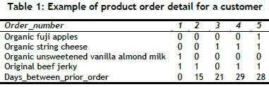
An example of how the 'days_between_orders_per_product' is calculated can be seen in Figure 8 for the product 'original beef jerky'. The symbol '|' indicates that the product was purchased with that order, and an 'O' indicates that the product was not purchased with that order. As can be seen, the user did not purchase the item with order 3. The corresponding days between product purchases can also be seen in the figure. The resulting sequence for 'days_between_orders_per_product' is thus [15 days, (21 days + 29 days) = 50 days, 28 days].

The last value of the sequence created in feature 1 is the target variable that must be predicted.

Feature 2: Days since prior order per product

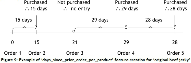
The 'days_since_prior_order_per_product' feature was created to capture some of the user's behaviour, along with the user-product behaviour. An example of how this feature is created, again for 'original beef jerky', can be seen in Figure 9. Assuming that the customer purchased the product, this feature evaluates how many days ago the user made a purchase (not necessarily the product that is being evaluated, but any product). As seen in the example, the product was purchased with order 2; thus the customer previously ordered 15 days ago, and the first entry for the sequence will be 15; but in order 3 this product was not purchased, so no record for this instance will be taken, as the product was not ordered. The product was again ordered with order 4; therefore an entry will be made, and the previous order was made 29 days ago. Thus the complete sequence in this example for the 'days_since_prior_order_per_product' will be [15,29,28].

These features were created for all user-product pairs in the dataset, and stored and used to derive non-sequence-based features from these sequences. These sequences were also used in the modelling phase. The structure of this new created dataset with its features can be seen in Figure 10. The non-sequence-based features that were created are described next.

3.3.2 Features that are not sequence-based but that describe the sequence

Some features were created to describe the sequence, but did not form a sequence themselves. These features were created for the XGBoost machine learning technique, as this technique looks at the bigger picture and not just at the user-product pair sequence.

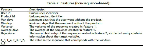
Table 2 lists all the non-sequence-based features that were generated, with a description to explain how the features were derived. Figure 11 shows how the dataset for the non-sequence-based features was created. Each user-product pair's last value of the sequence 'days_between_orders_per_product' is the target variable t0. The sequence was then split into windows with a size of six, each having five training examples in the sequence, with a value to predict as the sixth value. The last window was then separated into a test set. The other windows were flattened, which means that there is more than one user-product pair, and this creates the training set.

 

 

The sets were then further expanded with features derived from the five variables in the window.

These features are listed and explained in

Table 2. Each of these variables was created based on the five values in the window. For example, if the 'days_between_orders_per_product' sequence looked as follows:

[23,19,16, 24, 23, 28, 30, 12, 19, 27, 15, 21, 29],

the target variable t0 = 29,

the last window = 30, 12, 19, 27, 15, 21 (days) with 21 being the target variable for this window,

the second last window = 23,19,16, 24, 23, 28 (days) with being 28 the target variable for this window.

Figure 12 shows the final form of the training dataset, with all the features created.

3.4 Modelling

After the features and datasets had been created, the models were developed and tested. The first approach followed was to predict the NPD by using only sequence-based features. This was trained using an RNN, which is used for time series prediction and is explained in section 2.1.2.

3.4.1 RNN implementation

The RNN (see Section 2.1.2) was trained using only sequence-based features, as seen in Figure 10. The first implementation took the entire sequence of feature 1, except the last entry of the sequence to train the model and the last entry in the sequence as the test variable with which the prediction can be compared. The second implementation of an RNN model took the sequences of both feature 1 and feature 2. The target variable stayed the same (the last entry in the feature 1 sequence), and the last entry of both sequences was removed from the training. Thus the training set size was equal to the user-product pair sequence size without the last variable.

Because sufficient data was needed to train the model, the user-product pair was filtered to have at least 20 entries, thus leaving a dataset with 112 796 user-product pairs for NPD to predict.

The RNN was implemented in Python by using PyTorch, an open-source machine learning library. The sequences were scaled before training, with the parameters that could be set being the optimiser, the learning rate, the criterion, the number of hidden layers, and the activation function. The Adam optimiser was used with a learning rate of 0.01 and 10 hidden layers. A rectified linear unit (relu) activation function was used with a mean squared error loss criterion.

3.4.2 Regression implementation

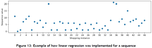
The second sequence-based approach (Section 2.1.3) was implemented by using linear regression. Figure 13 shows how the sequence data was represented for linear regression, with the shopping instance on the x-axis and the sequence value (days between purchases) on the y-axis. For this implementation, the next value of the shopping instance, in this case 47, was predicted.

The regression model was implemented in Python using the machine learning library Scikit-learn's SGDRegressor (SGD stands for 'stochastic gradient descent'). The data was scaled and the default parameters were used, with a squared loss function and a learning rate of 0.001.

3.4.3 XGBoost implementation

An approach to using not only sequence-based features was explored by training an XGBoost model (see Section 2.1.4) with the training set seen in Figure 12. This was done to see whether there was value in training data from other users as well.

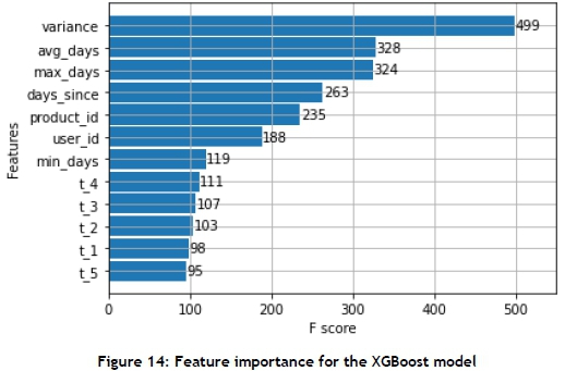
The feature importance can be seen in Figure 14. It is noticeable that the most important feature is the variance, followed by the user_id, which indicates that the model finds it important to know for which user it is predicting. Interestingly, the five features that indicate the sequence are least important, along with the minimum days that the customer goes without the product.

 

 

The XGBoost model was implemented by using the XGBoost package in Python with the following parameters (other parameters not mentioned were set to default):

Criterion: Root mean squared error

Learning rate: 0.1

Objective: reg:linear

Booster: gradient boosting tree

3.4.4 Neural network implementation

A neural network (NN) (see Section 2.1.1) model was trained with the same training set as the XGBoost model. The NN was trained with 12 input features (corresponding to 12 neurons in the input layer), one hidden layer with eight neurons, and the output layer with one neuron. A relu activation function was used with a mean squared error loss criterion and an Adam optimiser. The features were scaled before training the model.

After the models (XGBoost and NN) had been trained, the models were tested on the test set, and the absolute error was calculated by subtracting the prediction from the target variable and taking the absolute value.

3.5 Evaluation (results)

To evaluate the models, the absolute error in days was calculated for each user-product pair for each technique. The absolute errors were sorted from small to large and plotted, as seen in Figure 15. The graph on the left-hand side shows all the user-product pairs' absolute prediction errors. The NN implementation performs best, as it has the smallest absolute error over number of user-product pair instances. In the graph on the right-hand side, only the first 40 000 user-product pair instances are plotted. This shows that the NN has a much smaller gradient than the other techniques. This also shows that the NN can predict at least 40 000 user-product pairs with an absolute error of less than one-and-a-half days.

 

 

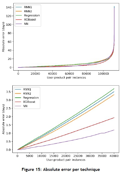
Figure 16 shows the number of user-product pairs per absolute error. It shows that the NN predicts a lot more NPDs with smaller errors than the rest of the algorithms, while XGBoost also outperforms the sequence-based approaches. Thus it can be said that the non-sequence-based algorithm outperforms the other algorithms in this instance. This also shows that looking at the bigger picture and not only at an individual user-product pair can be advantageous.

 

 

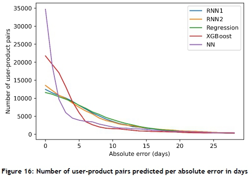
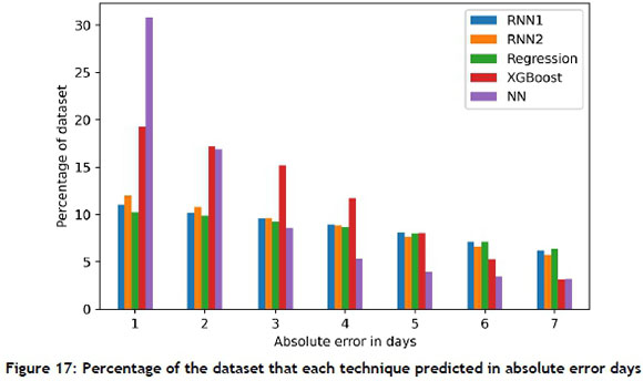
Figure 17 shows the percentage of the dataset that each algorithm predicted per category. The NN algorithm can predict the NPD with an error of less than one day for 31.8 per cent of the dataset, and another 16.8 per cent with an error of between one and two days. This outperforms all the other algorithms, with the next best algorithm, XGBoost, predicting 19.3 per cent with an error of less than one day. This also shows that the NN can predict more than 55 per cent of the user-product pairs with an error of less than three days.

 

 

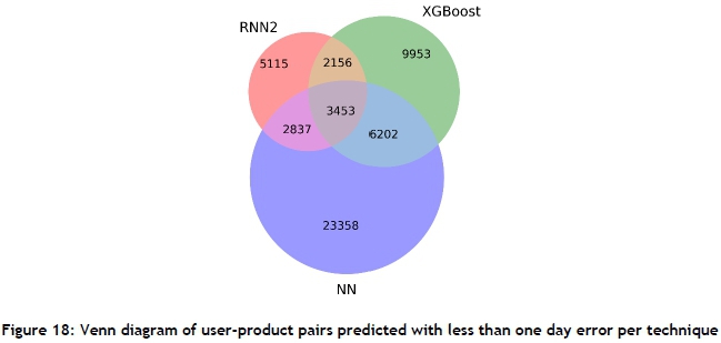
To see whether the algorithms performed well on the same user-product pairs, the user-product pairs from RNN2, XGBoost, and NN with errors of less than one day were plotted with a Venn diagram, which can be seen in Figure 18. This shows that only 3 453 of the total 53 074 pairs (6.5 per cent) were predicted with errors of less than one day by all three of the algorithms. Thus a combined approach could possibly increase the quality of the NPD predictions.

 

4 CONCLUSION

Predicting a user-product pair's next purchase date using machine learning is possible. It can be seen in this paper that using a technique that takes all the data into account, including data from other user-product pairs, performs better than the approach of predicting the NPD by only using the data of one user-product pair. The NN outperforms the other algorithms, with XGBoost performing second-best, which is better than all the sequence-based approaches.

Data is the new oil, and thus is a resource that must be carefully used and managed. It is natural, therefore, for industrial engineers to develop building blocks of systems to support business operations and decision-making with machine learning. This study shows how machine learning can be used to predict the next purchase date for an individual retail customer. A retailer can use the results to develop a system that offers individual customers personalised discounts on specific products on specific days. This concept differs from the typical loyalty programmes, since the offers are personalised, based on the individual customer's buying history. The NPD predictor is a system for the future and, once implemented, will reduce wasted paper inserts (typically found in newspapers), and may help a retailer to plan inventory better, which may save on logistics costs and reduce the pollution caused by distribution.

This study identifies opportunities for further work, including:

1. Extending the analysis to more datasets.

2. Deploying the NPD predictor at a retail chain using the NN algorithm.

3. Exploring ways to combine the sequence-based attempts with the non-sequence-based attempts.

4. Determining marketing strategies to target specific users, using the NPD predictor.

ORCID* identifier

M. Droomer: https://orcid.org/0000-0002-3782-1916

J. Bekker: https://orcid.org/0000-0001-6802-0129

 

REFERENCES

[1] Hosseini, M. & Shabani, M. 2015. New approach to customer segmentation based on changes in customer value. Journal of Market Analysis, 3(3), pp. 110-121.         [ Links ]

[2] Linoff, G.S. & Berry, M.J. 2011. Data mining techniques: For marketing, sales, and customer relationship management. Indianapolis: John Wiley & Sons.         [ Links ]

[3] Raorane A.A., Kulkarni, R.V. & Jitkar, B.D. 2012. Association rule - Extracting knowledge using market basket analysis. Research Journal of Recent Sciences, 1(2), pp. 19-27.         [ Links ]

[4] Cumby, C., Fano, A., Ghani, R. & Krema, M. 2005. Building intelligent shopping assistants using individual consumer models. IUI 05 - 2005 International Conference on Intelligent User Interfaces. San Diego, California, USA.         [ Links ]

[5] Cumby, C., Fano, A., Ghani, R. & Krema, M. 2004. Predicting customer shopping lists from point-of-sale purchase data. KDD '04 Seattle, Washington, USA.         [ Links ]

[6] Els, Z. 2019. Development of a data analytics-driven information system for instant, temporary personalised discount offers. M.Eng thesis, Stellenbosch University.         [ Links ]

[7] Mikolov, T., Karafiat, M., Burget, L., Cernocky, J. & Khudanpur, S. 2010. Recurrent neural network based language model. INTERSPEECH 2010, 11th Annual Conference of the International Speech Communication Association, Makuhari, Chiba, Japan, September 26-30, 2010.         [ Links ]

[8] Duda, R.O., Hart, P.E. & Stork, D.G. 2001. Pattern classification, 2^nd ed. New York: Wiley-Interscience.         [ Links ]

[9] Chen, T. & Guestrin, C. 2016. XGBoost: A scalable tree boosting system. In Proceedings of the ACM SIGKDD International Conference on Knowledge Discovery and Data Mining, (13-17), pp. 785-794. https://doi.org/10.1145/2939672.2939785.         [ Links ]

[10] Chapman, P., Clinton, J., Kerber, R., Khabaza, T., Reinartz, T., Shearer, C.R. & Wirth, R. 2000. CRISP-DM 1.0: Step-by-step data mining guide. CRISP-DM Consortium. Technical report.         [ Links ]

[11] Instacart. 2017. The Instacart online grocery shopping dataset 2017. [Online]. Available: http://https://data.world/datasets/instacart. [Accessed: 03-11-2020].         [ Links ]

 

 

* Corresponding author: jb2@sun.ac.za