GENERAL ARTICLES

 

Implementation of machine learning techniques for prognostics for railway wheel flange wear

 

 

C.J. Fourie^*; J.A. du Plessis

Department of Industrial Engineering, University of Stellenbosch, South Africa

 

 

---

ABSTRACT

Machine learning has become an immensely important technique for automatically extracting information from large data sets. By doing so, it has become a valuable tool in various industries. In this investigation, the use of machine learning techniques for the production of railway wheel prognostics was investigated. Metrorail's railway wheel wear data was used as a case study for this investigation. The goal was to demonstrate how machine learning can used on the data generated by Metrorail's routine operations. Three machine learning models were implemented: logistic regression, artificial neural networks, and random forest. The investigation showed that all three models provided prognoses with an accuracy of over 90 per cent, and had an area under curve (AUC) measurement exceeding 0.8. Random forest was the best performing model, with an AUC measurement of 0.897 and an accuracy of 93.5 per cent.

---

OPSOMMING

Masjienleer het 'n belangrike tegniek geword wanneer dit kom by die outomatiese ontginning van inligting uit groot datastelle. 'n Wye verskeidenheid van bedrywe het al voordeel getrek uit die implementering van masjienleer. In hierdie ondersoek was daar gekyk na hoe masjienleer gebruik kan word om prognostiese voorspellings te maak m.b.t. die verwering van spoorwegwielflense. Die doel van die ondersoek was om te demonstreer hoe masjienleer waarde uit Metrorail se data kan ontgin. Drie masjienleer modelle is geïmplementeer: logistiese regressie, kunstmatige neurale netwerke, en 'random forest'. Die resultate van die ondersoek het getoon dat al drie modelle 'n akkuraatheid van oor die 90 persent behaal het. Al drie modelle het ook 'n area onder die kromme (AUC) telling van meer as 0.8 behaal. Die 'random forest' model het die beste presteer van al drie die modelle, met 'n AUC telling van 0.897 en 'n akkuraatheid van 93.5 persent.

---

 

 

1 INTRODUCTION

Passenger railway services (PRS) are required to provide communities with punctual, safe, and affordable railway transport. The physical asset maintenance strategies that are implemented by PRS providers have a direct bearing on the punctuality, safety, and cost of the services they provide. A PRS provider's physical asset maintenance strategy must be cost-effective, and must uphold a high availability rate of its assets without sacrificing the diligence and quality of the maintenance work that is done.

It stands to reason that the maintenance management team of a PRS will greatly benefit from a prognostic decision support system. Such a system can predict when a system or component will fail, which informs maintenance teams about prioritising and scheduling their maintenance efforts. By enabling maintenance to be implemented on an 'as-needed' basis, a prognostic decision support system can aid in developing maintenance strategies that maintain the condition of assets, while reducing the cost associated with unnecessary maintenance efforts. By aiding maintenance management with maintenance planning, such a decision support system can also help to improve resource allocation decisions. These can increase the throughput rate of maintenance operations, which will lead to the higher availability of the assets being maintained.

The necessity of the advantages provided by prognostic decision support systems to PRS is especially high at Metrorail. Metrorail is a subsidiary of the Passenger Rail Agency of South Africa (PRASA), operating in the four main metropolitan areas of South Africa. The necessity stems from the fact that Metrorail employs an aging fleet of rolling stock, Metrorail's physical assets are frequently damaged or destroyed during acts of vandalism and theft, and a large portion of Metrorail's clients come from lower income groups who rely on Metrorail for their daily transportation needs. Even though this list of reasons is by no means exhaustive, it shows that Metrorail relies on a fragile system to provide a crucial service to a vulnerable portion of the South African population; hence the need for a prognostic decision support system to aid maintenance management.

Machine learning (ML) is an exciting field of study that focuses on developing computer programs that are capable of learning to perform tasks rather than being explicitly programmed to do so. ML techniques have been used to solve problems in various industries such as agriculture, healthcare, and marketing. In this article, the implementation of ML techniques to develop a prognostic decision support system for a PRS provider was investigated. As a case study, the techniques were applied to develop a prognostic model capable of producing prognoses for the railway wheels used by Metrorail. The findings presented in this article were used to serve as a proof-of-concept for the use of ML techniques to develop prognostic decision support systems that can aid maintenance management at Metrorail.

The following objectives were investigated:

1. To implement three ML models (logistic regression, artificial neural networks (ANN), and random forest (RF)) to provide railway wheel prognostics.

2. To implement methods of comparing the performance of the three model types.

3. To report on the best performing of the three model types.

 

2 LITERATURE REVIEW

2.1 Prognostics

The Oxford Learner's Dictionary [1] defines 'prognosis' as "a judgement of how something is likely to develop in the future". In the context of physical asset maintenance, a prognosis can refer to a prediction of the future state or condition of an asset. Tiddens, Braaksma and Tinga [2] highlighted the utility of a prognostic decision support system, in a physical asset maintenance context, by comparing it with a diagnostic system. The crux of the comparison was that prognostic techniques are prospective in nature, and therefore offer management the opportunity to pre-empt or prepare for asset failures. Diagnostic techniques, on the other hand, are retrospective in nature, and so provide information related to the cause and nature of a physical asset failure, but only after the failure has occurred.

Some of the most notable advantages of a prognostic decision support system in the context of physical asset maintenance have already been highlighted. These advantages stem, mainly, from the prospective nature of such a tool. Its main drawback lies in the difficulty of its development. The key element of any prognostic tool is a model capable of predicting the future state of its subject. Generally, these models are either physics-based or data-driven. A physics-based model consists of a mathematical representation of the subject and the processes that determine its future state. Formulating these mathematical expressions can be challenging, especially in the physical asset prognostics context, where the assets often consist of various interacting components, and where the degradation processes can be complex. Therefore the development of a physics-based model often requires knowledge and expertise that can be expensive to acquire [3].

With data-driven modelling, prognostic models are derived directly from routinely collected data for monitoring conditions. The key advantage of data-driven modelling over physics-based modelling is that data-driven modelling does not require the domain-specific knowledge and expertise that physics-based modelling does. However, data-driven modelling has a key requirement - the availability of a sufficiently sized repository of condition monitoring data - from which a prognostic model can be derived [4].

2.2 Machine learning

As stated, ML is focused on developing computer programs that are capable of learning. Mitchell [5] has stated that a computer learns as follows:

A computer program is said to learn from experience E with respect to some class of task T and performance P, if its performance at tasks in T, as measured by P, improves with experience E.

Two factors have contributed significantly to the growth in the popularity of ML. The first of these is the decreasing cost of computing power and data storage. The second is the fact that sensors capable of capturing data have become more affordable and available. The ubiquity of mobile phones that are equipped with highly sophisticated sensors and instruments supports this notion. These two factors have resulted in a rapid increase in the rate of data generation, which calls for new techniques that are capable of automatically extracting information from this data. ML is one such technique that provides this capability.

ML problems are usually subsumed under one of two categories: classification or regression. With the latter, the task of the ML model is to predict a continuous numerical value. Examples of regression problems include forecasting sales or predicting stock prices. With classification problems, the task of the ML model is to assign an observation to one of a set of categories. Examples of classification problems include the task of classifying a person as either male or female, based on their height and weight measurements. Another example of a classification problem is predicting whether a physical asset will be functional or non-operative at a future point in time, given its current state and working conditions [6].

Quite a few ML model types have been developed to solve classification problems. These model types will be referred to as classifiers in this article. Examples of popular classifiers are support vector machines, boosting algorithms, and decision trees. The classifiers that were implemented in this investigation were logistic regression, artificial neural networks (ANN), and random forest (RF).

2.2.1 Logistic regression

Logistic regression is a binary classifier that models the probability that an observation belongs to a specific category, based on a set of input features. The model takes the form P(X) = P(Y=1 |X), where X is a vector consisting of a set of input features, and Y is a binary target variable. The classifier takes, as input, a weighted linear combination of a set of input features, and returns a prediction of the probability that the observation belongs to a default binary class (Y = 1) [6], [7].

 

Figure 1

 

Logistic regression makes use of a link function that returns a value between 0 and 1 for all values of X. There are numerous functions that meet this description, but with logistic regression the logistic function is used; it is expressed as

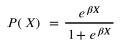
The variable ß in the logistic function is a vector of weights. With some manipulation, we find that the logistic function takes the form

which shows that the logistic regression model has log-odds that are linear in X.

The predictive performance of the model is improved by adjusting the vector of weights, ß. A popular method of optimising the model parameters is maximum likelihood estimation. The likelihood function has the form

In the likelihood function, each xi is an observation of the input data that belonged to class Y = 1, and for each xi, Y = 0. If ß is selected to maximise the likelihood function, it would mean that the logistic function is predicting values close to 1, for observations where the true class is 1 while predicting values close to 0 for observations where the true class is 0 [7].

2.2.2 Artificial neural networks

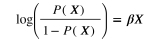
ANNs are a biologically inspired ML classifier that mimic the way in which the brain processes information. The brain has a large number of information processing units called neurons, which are interconnected by electrically conductive axons, as shown in Figure 2. In crude terms, information is ingested by the brain in the form of electrical impulses. An electrical impulse is conducted to a neuron from a large number of neighbouring neurons, via axons. If the combination of entering impulses exceeds some threshold, the neuron, in turn, fires an impulse through its axons to subsequent neurons. The brain's reaction to a stimulus comes in the form of a specific combination of firing neurons [8].

 

 

ANNs are conceptualised as a series of aggregating mathematical functions that constitute the artificial neurons, which relay their output via weighted connections to subsequent neurons. These weights represent the artificial axons of an ANN [9].

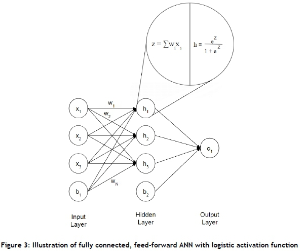
ANN configurations differ with respect to the aggregation functions (also known as activation functions) used for each neuron in the network, the number of neurons in the network, and the degree and manner of interconnectedness among neurons in the network. In this article, a common configuration for ANNs is used; a fully-connected, feed-forward ANN, which comprises three layers of neurons. The first layer is referred to as the input layer, which represents the raw input data, X, which is fed to the model. The second layer is referred to as the hidden layer, while the third layer is referred to as the output layer. The aggregate function used in both the hidden layer and the output layer is the logistic function, referred to in Section 2.2.1. The term 'fully connected' refers to the fact that the neurons in each layer of the network are connected to all neurons in the subsequent layer by a set of weights, W, as illustrated in Figure 3.

The advantage of ANNs stems from the interconnectedness of the neurons in the network, allowing it to model very complex behaviour. This becomes evident when we consider that a logistic regression model would represent a single node in an ANN. Therefore ANNs have an advantage over logistic regression models when modelling phenomena with complex behaviour. However, this complexity comes at a cost, and is the source of many of the disadvantages of ANNs.

First, ANNs are much more computationally expensive to optimise (also referred to as training) than logistic regression models. ANN training is achieved by making predictions on data for which the true target value is known. A measure of the difference between the predictions and the true values is then calculated; this is known as the prediction error. By exploiting the chain rule of partial differentiation, the change in the error with respect to a change in the value of each weight in the network is computed. In this way, the weights are incrementally adjusted, in order to reduce the overall predictive error of the model. This process, known as the backpropagation algorithm, is repeated until the performance of the model is deemed sufficient or the change in model performance diminishes [5], [9]. Backpropagation is computationally expensive, and scales poorly as the size of the ANN increases.

Second, ANNs are prone to over-training, which is a ML phenomenon: a model is trained to the point where it internalises the nuances of the training data that was used to train it. This inhibits the model's ability to make accurate predictions on data that was not present in the training dataset. This tendency to over-train is a consequence of the high variance exhibited by ANNs - that is, the ability of ANNs to model complex functions/behaviour.

Finally, ANNs are referred to as 'black boxes' because it is difficult to extract the rationale behind the predictions they produce. This is a disadvantageous characteristic of ANNs, especially when ML is implemented with the intention of gaining insights into the system or process that is being modelled.

2.2.3 Random forest

Random forest is a decision-tree-based ML model that reduces the high variance exhibited by conventional decision-trees, by building out and averaging over a large number (i.e., a 'forest') of decision-trees. A decision-tree classifier is built by successively dividing the input space of the problem into regions that exhibit high purity. A visual representation of a decision-tree is given in Figure 4 [7].

 

 

Figure 4 shows how each variable, X1 to X5, is successively divided until six distinct regions, known as leaf nodes, are formed. The purity of a leaf node refers to the extent to which it contains observations from only one of the members of the categorical output variable. A prediction is made by taking the mode class of the leaf node to which an observation belongs. With random forest, many decision-trees are built, using different combinations of subsets of the input variables; and each tree is built using a different randomly selected sample of the training data. The prediction of the model is then taken as the mode prediction made over all of the decision-trees [10].

Leaf purity is used to determine the sequence in which the input variables are split. The Gini impurity score is a measure of leaf impurity for a split produced by a given variable. The score is calculated as

The Gini impurity of a given variable (i) is calculated as a sum, over all M classes of the input variable, of the product of the proportion of observations with class M=m (pm) and the proportion of observations where class M=m with output variable class Y=k (pm,k). For a given value of pm, Gi is maximised when pm,k = 0.5, and minimised when pm,k=1. When a decision needs to be made about which variable should be selected to make the next split in a decision tree, the variable with the lowest Gini impurity score is chosen [7], [10]. The advantage of random forest models is that they are computationally inexpensive to train, yet are capable of modelling complex behaviour. And the classifier is quite resistant to over-training, especially if the number of trees that are generated is large, because the predictions that it produces are the result of averaging over a large number of predictions made by unique sub-models. The disadvantage of random forest models is that they become increasingly difficult to interpret as the number of trees in the model increases. Eventually, if a large enough number of trees are generated, the model can be considered to be a 'black box' that provides little insight into the process or system being modelled [7], [10].

The model parameters that are to be adjusted to improve its performance are the maximum tree depth (i.e., the number of splits per tree), the minimum leaf node size, the number of trees to grow, the number of observations to sample per tree, and the number of variables to sample per tree. These parameters are often optimised using an exhaustive grid-search approach.

 

3 CASE STUDY

3.1 Case description

The ML techniques discussed in Section 2 were implemented on railway wheel wear data, recorded by Metrorail, to provide flange wear prognostics. As stated in Section 2, one of the key requirements of ML is the availability of relevant data that can be used to train the ML models. The railway wheel condition monitoring data set represents one of Metrorail's most complete condition monitoring data sets.

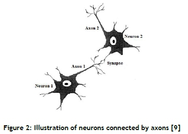
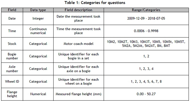
The data set consists of 454,187 records from between 2009-12-09 and 2018-07-05. A list of the fields is provided in Table 1. The data was recorded using a MiniProf railway wheel profile measurement instrument. A MiniProf mounted on a railway wheel is shown in Figure 5. This instrument was used during wheel condition monitoring inspections to measure wheel profiles. The wheel is decommissioned or sent for repairs when the flange height increases beyond 35mm.

 

 

Figure 6 illustrates how the flange height is affected by wheel wear. The figure shows the profile of a new wheel superimposed on the profile of a worn wheel. The relative height between the wheel tread and the apex of the wheel flange increases as the wheel becomes worn out. If this relative distance exceeds 35mm, the wheel is sent for repairs or is decommissioned. In Figure 7, note how the flange height of a sampled wheel position on the train develops over time. The flange height gradually increases to the point where the wheel is replaced. In the example provided, the wheel is replaced twice.

 

 

 

 

3.2 Feature engineering

To improve the performance of the ML models, some additional features were created. This process is referred to as 'feature engineering'. In total, six additional features were created.

3.2.1 Time between measurements

' Time between measurements' was defined as the time that passed between successive flange height measurements of a specific wheel, measured in days. This feature was created to serve as a proxy for the extent to which the wheel was used between measurements. This was necessary because the distance covered by a wheel between measurements was not available.

3.2.2 Wheel instance age

This feature was defined as the total age of a wheel, measured in days. The reasoning behind this feature was that, if flange height wear is a non-linear process, then the extent to which a wheel is worn for a specific period of use is dependent on the age of the wheel at the start of this period.

3.2.3 Relative flange height difference

Relative flange height difference was used to create three features that express the relative difference between the diameter of a wheel and its neighbouring wheels. The first of these was the flange height difference between a wheel and that of the opposing wheel mounted on the same axle. The second feature was the relative difference between a wheel's flange height and that of the wheel with the smallest flange height on the same bogie. Finally, a measurement was created to show the difference between the average flange height of a coach and that of the neighbouring coach with the smallest flange height. The reasoning behind this feature was that wheels with larger diameters (i.e., smaller flange heights) will carry a relatively larger portion of the weight of the train, and so will wear at a different rate than smaller wheels.

3.2.4 Moving average wear rate

Moving average wear rate was calculated as the average wear rate, for a wheel, over the past three flange height measurements that were taken for a wheel. The reasoning behind this feature was that the historical rate of deterioration for a given wheel will provide some indication of the expected rate at which the wheel will deteriorate in the near future.

3.2.5 Previous flange height measurement

This measurement was defined as the flange height value that was recorded for a given wheel during the previous wheel condition monitoring intervention. The feature was created simply because a wheel that is close to being decommissioned for flange height deterioration will be more likely to have exceeded its allowed extent of flange height wear at the time of the next condition monitoring intervention, as opposed to a new wheel that still has a relatively small flange height.

 

4 MODEL DEVELOPMENT

In this section the methods that were used to build the ML models will be briefly described. The free statistical software environment, R, was used for data manipulation and model development requirements. The processes that were completed to develop the ML models were:

• Data preparation

• Grid-search parameter setup

• ML model training

• ML model testing

4.1 Data preparation

Data preparation was done in three steps. First, records containing impossible values were removed from the data set. Impossible, in this case, referred to records containing negative flange heights or negative times and dates. Records were also not allowed to be future-dated, which in this case meant that dates were not allowed to be later than 2018-08-25, which was when the investigation took place. Finally, flange heights were not allowed to be greater than 50mm. This final constraint was set to allow for valid extreme values, because wheels were not strictly decommissioned or sent for repairs when their flange heights grew past 35mm.

The second data preparation process was to create the target variable for the ML models. This was achieved by appending a binary variable to the data set that had a value of 0 for observations where the flange height was below 35mm and a value of 1 if the flange height was higher than 35mm.

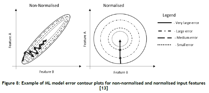
The final data preparation process is known as feature scaling. This process centres the mean of all numerical variables at 0 and transforms numerical variables to have unit variance. This is done to improve the training time of ML models. The performance increase stems from the fact that data sets often include variables that are on vastly different scales, which can be detrimental to the training time of an ML model. This is especially relevant to ML models that make use of a gradient descent approach to model optimisation, such as logistic regression and ANNs. Figure 8 shows how feature scaling (also known as feature normalisation) can shorten the path that a gradient descent algorithm has to take to optimise a model consisting of two input parameters.

4.2 Grid search parameter setup

Exhaustive grid-search was used to optimise the various hyper-parameters of the implemented ML models. This process entails creating a table of the values for the hyper-parameters that will be trialled for each of the ML models. These parameters, therefore, are optimised, in the sense that the best combination of the issued hyper-parameter values is selected, and therefore global hyper-parameter optimisation is not guaranteed.

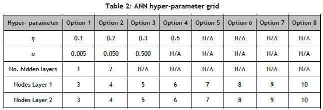
The term exhaustive refers to the fact that every possible combination of the hyper-parameters entered in the aforementioned table is tested to find the best-performing combination. The ANN hyper-parameters that were optimised in this way were:

• The learning rate (a)

• The momentum factor (n)

• The number of hidden layers

• The number of nodes per hidden layer

The random forest hyper-parameters were:

• The number of trees to generate (B)

• The number of features to sample when choosing a feature to split on (K)

• The number of observations to sample from the data set, per tree (L)

• The minimum allowed number of observations per leaf node (n)

The hyper-parameter tables (also referred to as grids) for the ANN and the random forest model are provided in Tables 2 and 3 respectively. The values that were selected for the tables were based on the default values selected for these parameters by the R packages that were implemented to build the models. A range of values centred on these default values were inserted into the hyper-parameter grids. No hyperparameters were adjusted for the logistic regression model.

4.3 ML model training

The first step in building the ML models was to split the data set into training and testing data sets. Seventy per cent of the prepared data set was randomly allocated for training purposes, and the remainder was held out for testing.

Each model (logistic regression, ANN, random forest) was built using an R package specifically designed to build its respective model. The base R package glm was used to build the logistic regression model. This package was designed for building a family of models called generalised linear models, of which logistic regression is a member. The following function call was used to build the model:

logistic_model = glm(train$target_variable~,family = binomial(link = "logit'),data = train)

The ANN2 package was used to build the ANN model, while the randomForest function of the ranger package was used to build the random forest model.

K-folds cross-validation was used while tuning the hyper-parameters. Five folds were used per configuration, and the average F1-score over the five folds was used to measure the configuration performance. The F1-score is a measurement of classifier performance, based on the metrics produced by confusion matrices.

The formula for the F1-score is:

The values TP, FN, and FP in the F1-score formula refer to true positive, false negative, and false positive classification rates respectively. The F1-score was used because it is computationally inexpensive to calculate, yet it produces classifier performance measurements that are less sensitive to target variable class imbalance than the conventional accuracy measurement. Figure 9 shows how the average F1-score over each of the five folds of the k-folds cross-validation process fluctuated over the trials of the various ANN hyper-parameter configurations. Figure 9 shows how some configurations performed worse than others.

 

 

The next performing ANN hyper-parameter configuration was a network with two hidden layers. It had eight nodes in the first layer and five nodes in the second. The value for a was 0.5 and the value for n was 0.1.

The winning hyper-parameters configuration for the random forest model was B = 550, no. features, no. observations and n = 9.

After the best hyper-parameter configurations were found, the ANN and random forest models were trained on the entire training data set.

4.4 ML model testing

The trained ML models were tested by having them predict whether a wheel will have exceeded its allowed flange height, based on the available cleaned and normalised input features. These predictions were made on the holdout data set to ensure the validity of the test.

One of the metrics used to measure the model's performance was area under curve (AUC), a metric derived from receiver operating characteristic (ROC) curves (see [10] and [14]). This metric was used because it is unaffected by target variable class imbalance. This was important because the occurrence of a wheel exceeding its allowed flange height was relatively scarce. The standard confusion matrix metrics - sensitivity, specificity, and accuracy - were also recorded for each model.

 

5 RESULTS

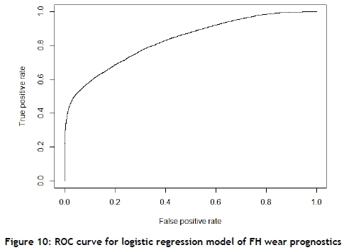
5.1 Logistic regression model performance

The ROC curve for the logistic regression model's predictions on the test data set is shown in Figure 10. The AUC for the model was 0.813. A confusion matrix of the predictions is provided in Table 4. The model had a sensitivity rate of 0.362, a specificity rate of 0.993, and an accuracy rate of 0.917.

 

 

5.2 ANN model performance

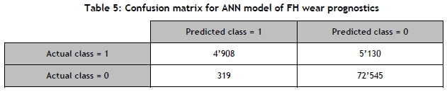
The ROC curve for the ANN model's predictions on the test data set is shown in Figure 11. The AUC for the model was 0.874. A confusion matrix of the predictions is provided in Table 5. The model had a sensitivity rate of 0.489, a specificity rate of 0.996, and an accuracy rate of 0.934.

 

 

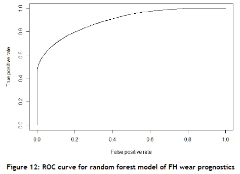
5.3 Random forest model performance

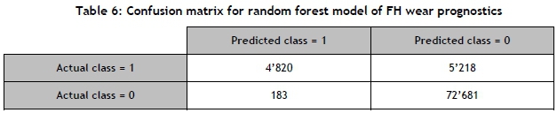
The ROC curve for the random forest model's predictions on the test data set is shown in Figure 12. The AUC for the model was 0.897. A confusion matrix of the predictions is provided in Table 6. The model had a sensitivity rate of 0.480, a specificity rate of 0.998, and an accuracy rate of 0.935.

 

 

6 CONCLUSIONS AND RECOMMENDATIONS

6.1 Conclusions

Three objectives were accomplished during the completion of this investigation. First, the three selected classifiers were implemented to provide railway wheel flange height prognostics. Second, three established methods of measuring and comparing the performance of the classifiers were implemented: ROC curves, AUC, and confusion matrix metrics. Finally, the three models were compared based on these performance metrics to select the best performing classifier.

The results reported in Section 5 showed that all three models performed well. All three models had an accuracy rate higher than 0.9 and an AUC measurement that exceeded 0.8. These scores indicate that all three models performed well. However, random forest marginally outperformed the other two classifiers.

A considerable portion of the accuracy reported for all three models stemmed from the imbalance in the target variable class, because the occurrence of a wheel flange exceeding its 35mm decommissioning height was quite rare. However, random forest had the highest specificity rate. This means that random forest was well suited for the detection of cases where the flange height exceeded 35mm. For these reasons, random forest was selected as the best-performing classifier in this investigation for flange height wear prognostics.

In conclusion, the data generated by Metrorail during its daily operations, such as condition monitoring operations, are of considerable value to various departments in Metrorail. This investigation showed that routinely collected wheel wear measurements can be used to build prognostic models that can provide insights and early asset failure warnings to maintenance management.

6.2 Recommendations

Although this investigation was able to achieve its purpose, it was not without limitations. First, it is reasonable to expect that the developed models could be improved if more data could be obtained from Metrorail. For instance, the distance covered by a specific train wheel would certainly add to the accuracy of wheel wear models. Second, reference is made in Section 1 to a range of additional classifiers. These could also be implemented on the provided data to determine whether better predictive performance could be attained. Third, a wider range of hyper-parameters could be tested to determine whether better performing models could be built.

In practical terms, it is recommended that the models developed in this investigation be implemented on a control set of actual railway wheels to determine how the models perform in a real-life setting. Finally, it is recommended that a follow-up investigation be launched to measure the possible financial impacts that prognostic models such as those developed in this investigation could have on Metrorail's maintenance operations.

 

REFERENCES

[1] Oxford Dictionaries. 2019. Prognostic. [Online]. Available: https://en.oxforddictionaries.com/definition/prognostic [Accessed: 05-Jan-2019].         [ Links ]

[2] Tiddens, W. W., Braaksma, A. J. J. & Tinga, T. 2015. The adoption of prognostic technologies in maintenance decision making: A multiple case study. Procedia CIRP, 38, pp. 171-176.         [ Links ]

[3] Elattar, H. M., Elminir, H. K. & Riad, A. M. 2016. Prognostics: A literature review. ComplexIntell. Syst., 2(2), pp. 125 - 154.         [ Links ]

[4] Solomatine, D. P. & Ostfeld, A. 2008. Data-driven modelling: Some past experiences and new approaches. Journal of Hydroinformatics, 10(1), pp. 3-22.         [ Links ]

[5] Mitchell, T. M. 1997. Machine learning. New York: McGraw-Hill.         [ Links ]

[6] Alpaydin, E. 2014. Introduction to machine learning. MIT press, 2004.         [ Links ]

[7] James, G., Witten, D., Hastie, T. & Tibshirani, R. 2013. An introduction to statistical learning. New York: Springer.         [ Links ]

[8] Basheer, I. A. & Hajmeer, M. 2000. Artificial neural networks: Fundamentals, computing, design, and application. J. Microbiol. Methods, 43(1), pp. 3-31.         [ Links ]

[9] Agatonovic-Kustrin, S. & Beresford, R. 2000. Basic concepts of artificial neural network (ANN) modeling and its application in pharmaceutical research. J. Pharm. Biomed. Anal. 22(5), pp. 717-727.         [ Links ]

[10] Marsland, S. 2015. Machine learning: An algorithmic perspective. New York: CRC Press.         [ Links ]

[11] Greenwood Engineering. n.d. MiniProf BT Wheel. [Online]. Available: https://www.greenwood.dk/miniprofbtwheel.php. [Accessed: 16-Sep-2018].         [ Links ]

[12] Shevtsov, I. Y., Markine, V. L. & Esveld, C. 2008. Design of railway wheel profile taking into account rolling contact fatigue and wear. Wear, 265(9-10), pp. 1273-1282.         [ Links ]

[13] Towards Data Science.2017. Gradient descent algorithm and its variants. [Online]. Available: https://towardsdatascience.com/gradient-descent-algorithm-and-its-variants-10f652806a3?gi=8cfd7ab31d6b. [Accessed: 10-Nov-2018].         [ Links ]

[14] Bradley, A. P. 1997. The use of the area under the ROC curve in the evaluation of machine learning algorithms. Pattern Recognit, 30(7), pp. 1145-1159.         [ Links ]

 

 

Submitted by authors 27 Feb 2019
Accepted for publication 18 /Mar 2020
Available online 29 May 2020

 

 

* Corresponding author: cjf@sun.ac.za