GENERAL ARTICLES

 

A case for implementing self-organising traffic signal control on South African roads

 

 

S.J. Movius^{*, #}; J.H. van Vuuren

Dept. of Industrial Engineering, Stellenbosch University, South Africa

 

 

---

ABSTRACT

Traffic signal optimisation may lead to the alleviation, to some extent, of urban traffic congestion, particularly by using real-time data rather than expected traffic flow data. Recent advances in radar technology have made it possible to observe detailed traffic flow data in and around roadway intersections in real time. The notion of self-organisation has relatively recently been proposed as a promising alternative to improve the effective allocation of green time, particularly under lighter traffic conditions. A fixed-time control strategy and seven self-organising algorithms are compared in a microscopic traffic simulation model of a provincial road in the Western Cape province of South Africa. Actual arrival rates are used as input for the model, while the algorithms are compared using six performance measure indicators, under both light and moderate traffic conditions. The results are used to make a case for the adoption of self-organising traffic signal control algorithms, especially under conditions of light to moderate traffic densities, since this can lead to significant improvements in traffic flow in terms of delay time, vehicle stops, and time spent travelling at unacceptably slow speeds through the road network.

---

OPSOMMING

Verkeerseinoptimering kan tot 'n mate die verligting van stedelike verkeersopeenhopings tot gevolg hê, veral deur gebruik te maak van verkeersvloeidata wat intyds versamel word, eerder as verwagte verkeersvloeidata. Onlangse ontwikkeling in radartegnologie het dit moontlik gemaak om gedetailleerde verkeersvloeidata in en rondom straatkruisings intyds waar te neem. Die konsep van self-organisasie is relatief onlangs as 'n belowende alternatief vir verbeterde doeltreffendheid in die toekenning van groenseintyd voorgestel, veral onder ligter verkeerstoestande. 'n Vastetydbeheerstrategie en sewe self-organiserende verkeersein beheeralgoritmes word in die konteks van 'n mikroskopiese verkeersimulasiemodel van 'n provinsiale pad in die Wes-Kaap provinsie van Suid-Afrika vergelyk. Werklike aankomstempo's word as insette vir die model gebruik, terwyl die algoritmes in terme van ses prestasiemaatstawwe vergelyk word, onder beide ligte en matige verkeerstoestande. Die resultate word gebruik om 'n saak te maak vir die aanvaarding van self-organiserende verkeerseinbeheeralgoritmes, veral onder toestande van ligte tot matige verkeersdigtheid, aangesien dit kan lei tot beduidende verbeterings in verkeersvloei as gevolg van verminderde vertragingstyd, die aantal kere wat voertuie stop, en tyd spandeer deur onaanvaarbaar stadig deur die padnetwerk te ry.

---

 

 

1 INTRODUCTION

Self-organisation is a relatively new approach to traffic signal control. It can be defined as the process by which a system becomes more ordered over a period of time as a result of interactions within the system itself rather than due to external control [1,2,3,4]. Self-organisation has the potential to lead to emergence, which occurs when the behaviour of a system exhibits unique characteristics that are not directly related to the elements at the lower level [1,4,5,6]. It has been claimed that self-organisation in urban traffic control may lead to an emergence of coordination between consecutive intersections, thus resulting in improved traffic flow as a result of the formation of more effective 'green waves' of unimpeded traffic flow [10].

In this paper, we provide empirical evidence in support of this claim. A fixed-time control strategy and seven self-organising algorithms are compared using a number of performance measure indicators (PMIs). The comparisons take place within the context of a microscopic traffic simulation model of the R44, a real corridor road network comprising eight signalised intersections in the Western Cape province of South Africa. Based on the results of this simulation comparison, we advocate that self-organising traffic signal control should be seriously considered as an alternative to current control measures during times of light to moderate traffic.

The paper is organised as follows. In Section 2, the logic of the standard fixed-time control strategy and that of seven self-organising algorithms are described. The microscopic traffic simulation model designed for use as a test bed in this paper is then described in Section 3. This description includes specifications of entities in the modelling framework, the model validation process, the output generated by the model, and the statistical analyses we perform on the model output data, as well as specific attributes of the real-world corridor under consideration. Simulation results obtained when implementing the eight signal control algorithms are presented in Section 4, under both light and moderate traffic conditions. Finally, a summary of the research conclusions is provided in Section 5.

 

2 ALGORITHMS

The logic of seven self-organising traffic signal control algorithms and of a standard fixed-time control strategy is described in this section. The self-organising algorithms all operate in real time and assume the presence of radar vehicle detection equipment, while the fixed-time strategy operates offline. The fixed-time control strategy (from here on referred to as 'Fixed') [7] is described first, followed by a description of a self-organising traffic single control algorithm proposed by Gershenson and Rosenblueth [8] (from here on referred to as 'Gersh'), an algorithm by Lämmer and Helbing [9] (from here on referred to as 'LH'), three algorithms proposed by Einhorn [10] that have been improved in a paper by Movius and van Vuuren [11] (referred to as the 'I-TSCA(n)', the 'O-TSCA(n)', and 'Hybrid(n)'), and finally two algorithms proposed by Movius and van Vuuren [11] (referred to as the 'VP-TSCA' and the 'SR-TSCA'). For more detailed descriptions of these algorithms, the reader is referred to the paper by Movius and van Vuuren [11].

2.1 The fixed-time control strategy

If a number of intersections are located relatively close to one another, it is desirable to coordinate their signal timings so that vehicles receive green signals as they reach consecutive intersections when travelling through the transportation network. This can be achieved by implementing a suitable cycle length, an offset time, and green times for various traffic movements through the intersections.

In this paper, the signal timings at each intersection are implemented in a cycle of length C, measured in seconds. The value of C is determined according to the optimal cycle length formula developed by Webster [7], which aims to minimise vehicle delays when considering random vehicle arrivals. This formula is given by

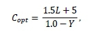
where L is the lost time per cycle (the sum of the setup times per cycle) and Y is the sum of the critical lane volumes divided by the saturation flow for each phase. In our simulation model, the appropriate cycle lengths are 50 seconds for light traffic conditions and 100 seconds for moderate traffic conditions.

2.2 The algorithm by Gershenson and Rosenblueth

The self-organising traffic signal control algorithm proposed by Gershenson and Rosenblueth [8] operates based on six rules that are ranked according to importance, with higher ranking rules overriding lower ranking rules. The algorithm uses a number of input parameters for which we select values recommended by Gershenson and Rosenblueth [8], unless otherwise stated.

The first rule states that, at each time step, the number of vehicles within a certain distance d (taken here as 50 metres) from an intersection that is currently not receiving service is tracked using a counter. If the counter exceeds a predetermined threshold value (taken here as 53.33 seconds), signals are changed and the counter is reset to zero. A minimum green time calculation is performed in the second rule. If this minimum green time has been exceeded, then the first rule is evaluated. Gershenson and Rosenblueth [8] recommended a very small value of 3.33 seconds, but we implemented a value of seven seconds; this is a more suitable (and recommended [12]) minimum green time. The third rule states that, if there are at most a small number of vehicles (taken here as 2) within a short distance (taken here as 25 metres) from the intersection in the same lane, signals may not change; while if there are more than two of these vehicles in the same lane within 25 metres of the intersection, the second rule is evaluated. The fourth rule states that, if there is at least one vehicle approaching an intersection within a distance d from an approach not currently receiving service, and there are no vehicles within the distance d from the intersection along an approach currently receiving service, the current green signal is terminated. If this is not the case, the third rule is evaluated. The fifth rule ascertains whether a spillback of vehicles into the intersection is imminent from a traffic flow currently receiving service. If there is at least one stationary vehicle within a short distance (taken here as 10 metres) beyond an intersection, the current green signal is terminated. Otherwise, the fourth rule is evaluated. The sixth and final rule is similar to the fifth rule, except that it takes into account all competing flows of traffic as opposed to only the flow currently receiving service. If at least one vehicle is stationary within the aforementioned distance beyond an intersection for all traffic flow directions, then all traffic directions receive a red signal, until some traffic flow direction no longer contains a stationary vehicle within that distance beyond the intersection. If, on the other hand, there are no stationary vehicles within the distance beyond the intersection for every traffic flow, the fifth rule is evaluated.

2.3 The algorithm of Lämmer and Helbing

The self-organising traffic control algorithm proposed by Lämmer and Helbing [9] was inspired by the observation of pedestrian flows at bottlenecks, and makes use of both a stabilisation strategy and an optimisation strategy. While each of these strategies has been reported to perform poorly under high traffic flow densities in isolation, it is known that they achieve a far better performance if they are combined appropriately, especially under lighter traffic conditions.

Lämmer and Helbing modelled traffic flow in a fluid-dynamic fashion, considering vehicle flow rates rather than individual vehicle speeds. It is therefore assumed in their model that all vehicles travel at a constant speed. By assuming vehicle arrival and departure rates, the expected number of vehicles to have reached an intersection by a certain time, as well as the number of vehicles expected to have departed from the intersection, can be determined, while the difference between the expected number of vehicles and the expected number of vehicles to have departed is equal to the number of vehicles that are expected to become queued.

The optimisation strategy of the algorithm relies strongly on the successful prediction of traffic flows in order to predict vehicle delays. This requires determining an appropriate amount of green time to clear a predicted queue, as well as the vehicles expected to join the queue during the setup time (amber and all red phases) and while the queue is being cleared.

A priority index

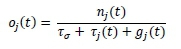
is assigned to traffic flow j, where jiy(t) is the number of queued vehicles along approach j at time t, τ_σis a penalty term incurred for terminating service to the current traffic flow (if j = σ , this term falls away), τ,-(ί) is the remaining setup time, and gj(t) is the green time. The approach achieving the largest priority index is awarded service.

The optimisation policy is employed while vehicle queues are bounded (i.e., remain below a certain threshold). The stabilisation policy of the algorithm, on the other hand, is employed if vehicle queues grow beyond a critical threshold, which is determined according to the threshold function

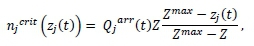
where n_j^critis the number of vehicles making up the critical threshold, Q_j^arr(t) is the arrival rate of vehicles along approach j, Ζ is the length of the desired interval in which each flow should be served once on average, Z^maxis the chosen maximum length of the service interval, and Zj(t) is the anticipated length of the service interval (the difference between the time at which the previous green time for approach j ended, and the start of the next green time it will receive). If the number of queued vehicles is larger than η_j^crit, that traffic flow immediately receives service until the traffic flow is no longer critical, at which point the optimisation strategy is restored.

2.4 The modified osmosis traffic signal control algorithm

The osmosis traffic signal control algorithm (O-TSCA) was originally put forward by Einhorn [10], but modifications to this algorithm were proposed by Movius and van Vuuren [11] to rectify some of its shortcomings. The modified version of this algorithm is referred to as the O-TSCA(n).

The algorithm was inspired by the chemical process of osmosis. Osmosis occurs when solvent molecules pass through a semi-permeable membrane from a lower solute concentration to a higher solute concentration due to the difference in pressure of the two solutions. A number of parallels may be drawn between the elements of osmosis and traffic control. The approaching vehicles that pass through an intersection are analogous to the solute molecules, while the intersection itself is interpreted as the semi-permeable membrane. The vacant space on the opposite side of the intersection represents the pull pressure exerted by the solute molecules on the solvent molecules (or vehicles) through the semi-permeable membrane (or intersection).

The O-TSCA(n) functions by first tracking the demand and availability of traffic flows. The demand is calculated by summing the effective lengths of approaching vehicles that are within 110 metres of an intersection, while the availability is the available space that may be occupied by vehicles on the opposite side of the intersection. This distance was proposed, instead of the original distance of 275 metres (range of the detection equipment), since it was found to be beneficial to consider only vehicles within a closer proximity to the intersection. Each traffic flow is then associated with a pressure, which is calculated as the sum of the demand and the availability. A traffic flow receives uninterrupted service either until the vehicle throughput exceeds the initial demand that was present at the start of service, or until the vehicle throughput exceeds the initial availability that was present at the start of the service interval. Once the vehicle throughput has exceeded any one of these initial values, the pressures of the competing traffic flows are compared, and the traffic flow corresponding to the largest pressure receives service, on condition that there are no approaching vehicles receiving service that are within 20 metres of the intersection.

2.5 The modified inventory traffic signal control algorithm

The original inventory traffic signal control algorithm (I-TSCA) was also put forward by Einhorn [10], with modifications again proposed by Movius and van Vuuren [11] in order to rectify some of the algorithm's deficiencies. The modified version of this algorithm is referred to as I-TSCA(n).

The I-TSCA(n) is based on the theory of inventory control, and attempts to minimise certain 'costs' associated with traffic control, such as delay time. The I-TSCA(n) iterates through three main steps, the first of which involves determination of the required green time. This green time is calculated as the amount of time required to clear the longest vehicle queue within a 110 metre distance from the intersection. If there is no vehicle within this distance from the intersection, the green time required by the closest vehicle to reach the intersection is used instead. This distance of 110 metres was proposed for the same reason as for the O-TSCA(n) above. During the second step, the vehicle delays associated with awarding service to a particular phase are calculated. The third step involves assigning green time to the traffic flow that results in the smallest total vehicle delay.

2.6 The modified hybrid algorithm

The original hybrid algorithm, 'hybrid', also due to Einhorn [10], combined the original O-TSCA and I-TSCA. The modified algorithm, referred to here as 'Hybrid(n)', is similarly a combination of both the O-TSCA(n) and the I-TSCA(n).

Hybrid(n) executes both the O-TSCA(n) and the I-TSCA(n) concurrently, while monitoring whether or not there is at least one vehicle within a vehicle's safety distance from the intersection. Once the I-TSCA(n) requests a signal change, Hybrid(n) continues awarding service either until the O-TSCA(n) also requests a signal change, or until there is no vehicle within a vehicle's safety distance from the intersection.

2.7 The vehicle platoon traffic signal control algorithm

The vehicle platoon traffic signal control algorithm (VP-TSCA) was proposed by Movius and van Vuuren [11]. The algorithm clusters vehicles into platoons according to their distances from one another. The algorithm aims to switch signals so as not to separate the platoons, by only executing a signal change once the distance between consecutive vehicles is larger than an inter-vehicle threshold distance. If two vehicles are within the inter-vehicle threshold distance from one another, they are considered part of the same platoon. This threshold distance is calculated based on the level of traffic congestion, which is measured according to the current road saturation. The road saturation χ and the inter-vehicle threshold distance D are assumed to satisfy the inversely proportional relationship

where a > 0 is a constant of proportionality, and b > 0 is an offset constant. Extensive numerical simulation experiments carried out by the authors have suggested that good values for the constants a and b are 2 and 10 respectively for the case study road network. This algorithm also makes use of a spill-back mechanism by terminating a green signal if vehicles begin backing up into the intersection.

2.8 The saturation ratio traffic signal control algorithm

The saturation ratio traffic signal control algorithm (SR-TSCA), also proposed by Movius and van Vuuren [11], aims to switch signals based on the ratios of road saturation of competing traffic flows. Once the ratio of current road saturation to the competing road saturation is smaller than a certain saturation ratio threshold parameter, given that a minimum green time has elapsed, signals are switched. The saturation ratio threshold Τ is related to the road saturation χ by the equation

where c > 0 is a constant of proportionality and d > 0 is an offset constant. Once again, extensive numerical simulation experiments were carried out. The results suggested that good values for the constants c and d are 15 and 0.23 respectively for the case study road network.

The minimum green time employed by this algorithm is calculated as the time required to clear all currently queued vehicles. Thereafter the signals switch once the current ratio of traffic flows drops below the saturation ratio threshold. A spillback mechanism is again employed to ensure that vehicles do not back up and block intersections.

 

3 THE SIMULATION MODEL

A newly designed microscopic traffic simulation model employed as a test bed in this paper is described in this section. This discussion includes the general specifications of a replicated real corridor road network, and the details of the model output and the statistical tests performed.

One prerequisite of the self-organising algorithms of Section 2 is the presence of radar vehicle detection equipment mounted at each intersection that can detect vehicle speeds as they approach an intersection and their distances from the intersection in each direction. The SmartSensor advance extended range radar detection unit [13] is the assumed mode of detection in this study, and is able to detect vehicles up to a distance of 275 metres away.

3.1 General specifications of the modelling framework

The road network topology considered in this paper is an eight-intersection corridor consisting of non-uniform intersections, shown in Figure 1 and modelled in Anylogic 7.3.5. The arrival rates of vehicles entering this network were recorded on a Tuesday in April 2013 during 15-minute intervals from 06:00 to 18:00 by the Department of Civil Engineering at Stellenbosch University [14]. These arrival rates were aggregated into one-hour intervals, and specific intervals were used as input for the model in order to mimic certain periods of traffic flow. The first interval includes arrival rates associated with the one-hour 06:00-07:00 period, which represents a very light traffic flow. The second interval includes arrival rates for the 10:00-12:00 two-hour period, representing a moderate traffic flow. The reason that very high traffic flows (such as those found during morning and afternoon peak times) are not considered is because self-organisation offers flexibility that is more suitable for traffic conditions that are not saturated.

Once a vehicle is generated within the simulation model, its destination is immediately known, and it travels the shortest (legal) route to reach its destination. Vehicles are assigned a length of five metres, and acceleration and deceleration rates are taken as the values recommended by Anylogic [15] - 1.8 m/s and 4.2 m/s respectively. A vehicle changes lanes if another vehicle travelling at a slower speed is detected ahead of it, or if the vehicle has an upcoming turn and is not currently in the required lane, while the preferred speed of a vehicle is uniformly distributed within the range 47-72km/h.

3.2 Model validation

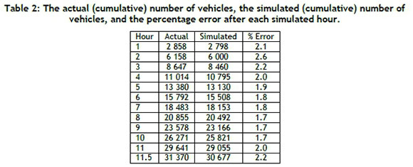
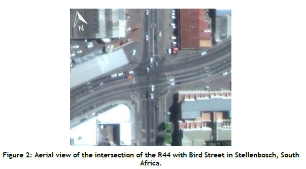
This simulation model was validated by comparing the output generated by the model with that of the real system in Figure 1. In a study carried out by Van der Merwe [16], real data were collected for one of the signal controlled intersections above (the intersection connecting the R44 and Bird Street, labelled '7' in Figure 1). The data captured included the number of vehicles and their associated manoeuvres through the intersection, as well as the green times granted by the signals at the intersection. The arriving vehicles recorded during the 15-minute intervals were aggregated into eleven one-hour periods and one half-hour period, while the green times were averaged into morning, midday, and afternoon green times. An image of the intersection is shown in Figure 2, and the green phases and the associated averaged green times captured by Van der Merwe [16] are shown in Figure 3 and Table 1 respectively.

 

 

The intersection in Figure 2 was replicated in Anylogic [15], and the aggregated green times, vehicle arrival rates from the study by Van der Merwe [16], and vehicle movements through the intersection were taken as input to the model. The model was executed 30 times for 11.5 simulated hours, and the output was recorded after each hour. These output data were compared to the actual output recorded in the Van der Merwe study [16], and the absolute errors were noted. The total number of simulated vehicles was, at most, only 2.6 per cent less than the actual recorded value shown in Table 2, indicating that the model accurately depicts a real-world system. The model was thus considered accurately calibrated and duly validated.

 

 

3.3 Model output

The data obtained from the radar detection units assumed to have been installed at each of the intersections in the study area are used in the signal switching decisions, and in calculating output data emanating from the simulation model. Once a warm-up time of 1800 seconds had elapsed, six PMI values - used to compare the relative performances of the algorithms - were recorded for each algorithm.

The first two PMIs are the mean delay time (PMI 1) and the normalised mean delay time (PMI 2) experienced by vehicles in the road network. The delay time is calculated by subtracting the ideal travel time of a vehicle (the route distance divided by the preferred speed of the vehicle) from the true time actually spent by the vehicle in the system (measured in seconds). The normalised mean delay time is calculated as the ratio of the mean delay time to the distance travelled by the vehicle to take into account any variation in the distances travelled by vehicles (a vehicle travelling further is more likely to experience a larger delay than a vehicle that travels only a short distance). If, for example, a vehicle achieves a normalised mean delay value of 2.0, this indicates that a vehicle has spent twice as long in the network than it would have had it travelled unimpeded at its preferred speed the entire way.

The next two PMIs are the mean number of stops (PMI 3) and the normalised mean number of stops (PMI 4) experienced by vehicles in the system. The latter PMI is calculated as the ratio of the mean number of stops of a vehicle to the number of intersections encountered by the vehicle during its route through the network. If a normalised mean number of stops achieves a value of 0.5, for example, this indicates that a vehicle is expected to have stopped at 50 per cent of the intersections it encountered.

The final two PMIs are the mean time vehicles spend travelling unacceptably slowly (taken here as under 10km/h and measured in seconds) and the normalised mean time vehicles spend travelling slowly (again under 10km/h), referred to as PMI 5 and PMI 6 respectively. The latter PMI is a ratio, calculated by dividing the mean time vehicles spend travelling under 10km/h by the total time the vehicle spends in the system, in order to capture the average portion of time a vehicle spends travelling unacceptably slowly. The value of 10km/h was chosen because it is slow enough for drivers to be in first gear and thus feel frustration while driving.

3.4 Statistical comparison methodology

Once the six PMIs had been recorded for 30 simulation runs, an ANOVA test¹ [17] was performed for each of the mean PMI values to determine whether there is a statistical difference between at least two of the algorithms' performances. If a statistical difference was detected, a Levene's test [18] was carried out to determine whether the variances between the PMI values returned by the algorithms were significantly different at a five per cent level of significance. If this was not the case, Fisher's least significant difference (LSD) post-hoc test [19] was performed to determine between which pairs of PMIs statistical differences were detectable. If, on the other hand, the variances were significantly different, a Games-Howell post-hoc test [20] was performed for this purpose instead.

 

4 ALGORITHMIC RESULTS

The arrival rates described in the previous section were taken as input data for the simulation model. The model was run for a single simulation hour between 06:00 and 07:00 (light traffic), and again for a period of two simulation hours between 10:00 and 12:00 (moderate traffic), as mentioned. The relative performances of the algorithms were recorded for the six PMI values returned over these specific time intervals to capture the state of the road network during the very low traffic demands of the early morning, and the moderate traffic experienced just before midday. The results of these simulations are reported and interpreted in the remainder of this section.

4.1 Light traffic conditions

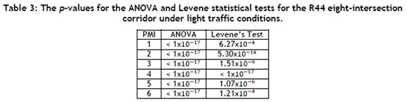
The ANOVA column in Table 3 indicates that, for all six PMIs, statistical differences were detected between the PMI means returned by the algorithms at a five per cent level of significance under light traffic conditions. Furthermore, applying the Levene test revealed that the algorithmic variances of the PMI mean samples were statistically distinguishable for all six PMIs, and so the Games-Howell post-hoc test was used to determine between which pairs of algorithmic outputs differences were statistically discernible for these six PMIs. The mean PMI values for each algorithm are given in Table 4, while the corresponding box plots are shown in Figure 4.

 

 

 

 

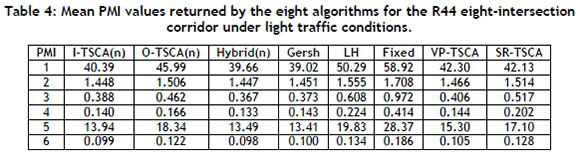
The best performances for mean and normalised mean delay were returned by Gersh, Hybrid(n) and the I-TSCA(n), while the performances of these three algorithms were statistically indistinguishable at a five per cent level of significance. The VP-TSCA and the SR-TSCA achieved the next best mean delay values of 42.30 seconds and 42.13 seconds respectively, and the VP-TSCA and the O-TSCA(n) achieved the next best normalised mean delay values of 1.466 and 1.448 respectively, although both pairs of algorithms returned statistically indistinguishable PMI means at a five per cent level of significance. LH was outperformed by all the other algorithms, with the exception of Fixed, for both mean and normalised mean delay.

Once again Gersh, Hybrid(n), and the I-TSCA(n) achieved the most favourable results for both mean and normalised mean number of stops, followed closely by VP-TSCA. The O-TSCA(n) was the next best performing algorithm in both these respects, achieving a normalised mean number of stops value of 0.166, indicating that vehicles under the control of the O-TSCA(n) are likely to stop at about 17 per cent of the intersections they encounter. Once again a relatively poor performance was exhibited by LH and Fixed, as well as by the SR-TSCA, for mean and normalised mean number of stops - further evidence of previous claims that these algorithms do not offer appropriate control under light traffic conditions.

Unsurprisingly, Gersh, Hybrid(n), and the I-TSCA(n) obtained the best results for the remaining two PMI values. The next best performing algorithm in both instances was the VP-TSCA, which achieved mean and normalised mean time spent travelling under 10km/h values of 15.30 seconds and 0.1054 seconds respectively. These values indicate that when the VP-TSCA is employed at signalised intersections, vehicles spend about 15 seconds of their journey travelling at very slow speeds, which amounts to roughly 11 per cent of their total time spent in the road network.

4.2 Moderate traffic conditions

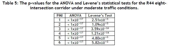
The ANOVA column in Table 5 indicates that, again, for all six PMIs there were statistical differences between the means returned by the various algorithms at a five per cent level of significance under moderate traffic conditions. Furthermore, the outcome of the Levene test revealed that the algorithmic variances of the mean samples were statistically indistinguishable for PMI 6, and therefore the Fisher LSD post-hoc test was used to determine between which pairs of algorithmic outputs differences were statistically discernible for this particular PMI. The Games-Howell post-hoc test was used for this purpose for the remaining five PMIs, as the Levene test indicated that there were statistical differences between the variances of the samples for these PMIs at a five per cent level of significance. The mean PMI values for each algorithm are given in Table 6, while the corresponding box plots are shown in Figure 5.

 

 

 

 

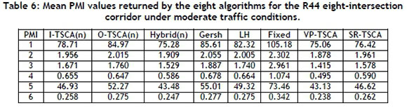
The VP-TSCA was not outperformed by any other algorithm for the mean and the normalised mean delay, achieving values of 75.06 seconds and 1.878 respectively. The VP-TSCA outperformed all other algorithms for the mean delay - except for Hybrid(n) and the SR-TSCA, from which it did not differ significantly - while significantly outperforming all the other algorithms for the normalised mean delay at a five per cent level of significance. For the normalised mean delay, Hybrid(n) was the next best performing algorithm, achieving a value of 1.909, indicating that vehicles spend, on average, an additional 91 per cent of their time in the road network as a result of delays.

A similar ranking was apparent for the mean and normalised mean number of stops. The VP-TSCA significantly outperformed all the other algorithms for these two PMIs, followed by Hybrid(n) and the SR-TSCA, whose performances did not differ statistically from one another at a five per cent level of significance. The I-TSCA(n), the O-TSCA(n), Gersh, and LH all achieved very similar results for these two PMIs, not differing statistically from one another for PMI 3 or PMI 4 at a five per cent level of significance. Fixed returned the poorest results, with vehicles stopping about twice as many times compared with the other seven algorithms.

The VP-TSCA outperformed all the other algorithms, except for Hybrid(n), from which it did not differ significantly for the mean time spent travelling under 10km/h. The I-TSCA(n) and the SR-TSCA achieved the next best results for this measure, followed by LH, which is ranked fifth. The VP-TSCA outperformed all the other algorithms for the normalised measure of time vehicles spend travelling slowly, achieving a value of 0.2381, implying that vehicles spend about 24 per cent of their time in the road network travelling at a maximum speed of 10km/h. Hybrid(n) obtained the next best result with a value of 0.2465. The I-TSCA(n) achieved the third best result for this measure, followed by the O-TSCA(n), Gersh, and LH, whose performances did not differ statistically from one another at a five per cent level of significance.

 

5 CONCLUSION

The results returned by the algorithms under light traffic conditions are not surprising, and corroborate statements reported by previous authors [11]. For instance, it was discovered [11] that the I-TSCA(n), Hybrid(n), and Gersh are particularly effective under light traffic conditions in the context of hypothetically constructed road networks (although not as light as in this scenario). Similarly, it was found that algorithms such as Fixed, LH, and the SR-TSCA are more effective under heavier traffic conditions, which explains their poor performance here.

The VP-TSCA was undoubtedly the best performing algorithm overall under moderate traffic conditions, as it was not outperformed by any other algorithm for any of the six PMIs. The VP-TSCA has therefore been shown to perform relatively well under very light, light, and moderate traffic conditions [11], indicating that the performance of this algorithm is rather robust with respect to the prevailing traffic conditions. This is attributed to the hyperbolic function relating to the road saturation level and the inter-vehicle threshold distances associated with the VP-TSCA logic, facilitating adaptation of its behaviour based on the current level of traffic congestion. Hybrid(n) is the next best algorithm under moderate traffic conditions, performing on a par with the VP-TSCA for two of the six PMIs, and ranking second best for the remaining four PMIs. The results returned by the SR-TSCA and the I-TSCA(n) are indistinguishable from one another for any of the six PMIs at a five per cent level of significance, and are the next best performing algorithms. Fixed returned the worst results for all six PMIs, which is not surprising, as it is better suited to heavier traffic conditions. This poor performance is largely attributed to the fact that the spacing between consecutive intersections is not uniform in the road corridor, and that the traffic flow densities at various intersections vary. This hinders the formation of green waves of traffic flow through consecutive intersections under a fixed traffic signal control regime, resulting in an increased number of vehicle stops.

In South Africa, Fixed is the most common form of traffic signal control. It is known to work well under very heavy traffic conditions, or when exact arrival rates are known, although this is never the case in reality. The results of this study indicate that the VP-TSCA obtained the best results, on average, for the real road corridor along the R44 under light and moderate traffic volumes. While the exact green times awarded by the real traffic signals at the eight intersections along the R44 are not known, they are expected to be close to those calculated using Webster's formula [7]. Therefore, by implementing self-organising algorithms such as the VP-TSCA, together with installing the necessary radar detection equipment, we have shown that a large saving in terms of delay time and vehicle stops can be achieved along the R44. This may be considered circumstantial evidence in support of a claim that the implementation of self-organising traffic signal control should be seriously considered during times of light to moderate traffic volumes on urban roads in South Africa.

 

6 ACKNOWLEDGEMENTS

The first author is indebted to the South African National Research Foundation (NRF) and the Harry Crossley Foundation for research funding.

 

REFERENCES

[1] De Wolf, T., Holvoet, T. & Samanaey, G. 2005. Engineering self-organising emergent systems with simulation-based scientific analysis. Proceedings of the 3^rd International Workshop on Engineering Self-Organising Applications, New York (NY), pp. 146-160.         [ Links ]

[2] Heylighen, F. 2001. The science of self-organization and adaptivity. The Encyclopedia of Life Support Systems, 5(3), pp. 253-280.         [ Links ]

[3] Serugendo, G.D.M., Gleizes, M. & Karageorgos, A. 2006. Self-organisation and emergence in MAS: An overview. Informatica, 30(1), pp. 45-54.         [ Links ]

[4] Shalizi, C.R. 2001. Casual architecture, complexity and self-organization in the time series and cellular automata. PhD thesis. Madison, WI: University of Wisconsin.         [ Links ]

[5] Heylighen, F. 1989. Self-organization, emergence and the architecture of complexity. Proceedings of the 1^st European Conference on System Science, Stuttgart, pp. 23-32.         [ Links ]

[6] Odell, J. 2002. Agents and complex systems, Journal of Object Technology, 1(2), pp. 35-45.         [ Links ]

[7] Webster, F.V. 1958. Traffic signal settings. Unpublished technical report. London: Road Research Laboratory.         [ Links ]

[8] Gershenson, C. & Rosenblueth, D.A. 2012. Adaptive self-organization vs static optimization: A qualitative comparison in traffic light coordination. Kybernetes, 41(3), pp. 386-403.         [ Links ]

[9] Lämmer, S. & Helbing, D. 2008. Self-control of traffic lights and vehicle flows in urban road networks. Journal of Statistical Mechanics: Theory and Experiment, 2008(4), pp. 1-30.         [ Links ]

[10] Einhorn, M.D. 2015. Self-organising traffic control algorithms at signalised intersections. PhD thesis. Stellenbosch: Stellenbosch University.         [ Links ]

[11] Movius, S.J. & van Vuuren, J.H. 2017. The effectiveness of self-organisation in signal control algorithms under light traffic conditions (submitted). Transportation Research Boards Part C: Emerging technologies.         [ Links ]

[12] Koonce, P. Rodegerdts, L., Lee, K., Quayle, S., Beaird, S., Braud, C., Bonneson, J., Tarnoff, P. & Urbanik, T. 2008. Traffic signal timing manual. Unpublished technical report. Portland, OR: Transportation and Research Board.         [ Links ]

[13] Wavetronix. 2016. Wavetronix SmartSensor Advance. [Online], cited March 23^rd 2016. Available from http://wavetronix.com/en/products/smartsensor/advance.         [ Links ]

[14] Department of Civil Engineering. 2013. Stellenbosch traffic signals. Unpublished technical report. Stellenbosch: Stellenbosch University.         [ Links ]

[15] AnyLogic. 2016. Multimethod simulation software. [Online], cited May 30^th 2016, Available from http://www.anylogic.com.         [ Links ]

[16] Van der Merwe, E. 2009. Improving the flow of an isolated traffic system. MA thesis. Stellenbosch: Stellenbosch University.         [ Links ]

[17] Hilton, A. & Armstrong, R. 2010. One-way analysis of variance. Hoboken, NY: John Wiley & Sons.         [ Links ]

[18] Schultz, B.B. 1985. Levene's test for relative variation. Systematic Biology, 34(4), pp. 449-456.         [ Links ]

[19] Williams, L.J. & Abdi, H. 2010. Fisher's least significant difference (LSD) test. Encyclopedia of Research Design, pp. 1-5.         [ Links ]

[20] Howell, J.F. & Games, P.A. 1974. The effects of variance heterogeneity on simultaneous multiple-comparison procedures with equal sample size. British Journal of Mathematical and Statistical Psychology, 27(1), pp. 72-81.         [ Links ]

 

 

Submitted by authors 14 Feb 2018
Accepted for publication 30 Jul 2019
Available online 30 Aug 2019

 

 

* Corresponding author: sjmovius@gmail.com
# Author was enrolled for a PhD in the Department of Industrial Engineering, Stellenbosch University, South Africa
1 Using aX-goodness of fit test, it was determined with 95% confidence that all the PMI samples returned by the algorithms were approximately normally distributed.