GENERAL ARTICLES

 

Single-machine scheduling of indivisible multi-operation jobs

 

 

F.C. Çetinkaya^{I, *}; H.A. Çatmakaş^I; A.K. Görür^II

^IIndustrial Engineering Department, Çankaya University, Turkey
^IIComputer Engineering Department, Çankaya University, Turkey

 

 

---

ABSTRACT

This paper considers a single-machine scheduling problem of multi-operation jobs where each job consists of several operations processed contiguously, rather than being intermingled with the operations of different jobs. That is, the jobs are indivisible. A sequence-independent setup is required if the machine switches from one operation to another. However, no setup is necessary before the first operation of a job if this first operation is the same as the last operation of the immediately previous job. A job is complete when all of its operations have been processed. We investigate the problem for two cases. Makespan, which is the time needed to complete all jobs, is minimised in the first case; whereas the total completion time, which is the sum of the job completion times, is minimised in the second case. We show that the makespan problem is solvable in polynomial time. For the problem of minimising total completion time, we develop a mixed integer linear programming (MILP) model, which is capable of solving small and medium-sized problem instances optimally, and obtain a very small gap between the solution found and the best possible solution for the unsolved large-sized problem instances.

---

OPSOMMING

Hierdie artikel ondersoek 'n enkel-masjien skeduleringsprobleem van meervoudige operasie take waar elke taak uit verskeie operasies bestaan wat kontinu verwerk word eerder as om gemeng te wees met die operasies van ander take. Die take is dus onverdeelbaar. 'n Volgorde-onafhanklike opstelling word vereis as die masjien wissel van operasie na 'n ander. Geen opstelling is egter nodig voor die eerste operasie van 'n taak indien die eerste operasie van die nuwe taak dieselfde is as die vorige taak se laaste operasie nie. Die tyd wat dit neem om elkeen van die take te voltooi is eerstens geminimeer. Daarna is die totale voltooi tyd (die som van al die taak voltooi tye) geminimeer. Daar word gewys dat die tyd wat dit neem om elke taak te voltooi oplosbaar is in polinome tyd. Om die totale voltooi tyd te minimeer is 'n gemengde heelgetal lineêre programmeringmodel ontwikkel wat daartoe in staat is om klein- en mediumgrootte probleme optimaal op te los. Die model behaal ook 'n baie klein verskil tussen die geïdentifiseerde oplossing en die beste moontlike oplossing vir groot probleemgevalle.

---

 

 

1 INTRODUCTION

Scheduling is the allocation of resources to complete a given set of tasks over time. In manufacturing systems, resources and tasks are usually referred to as machines and jobs respectively [1]. Scheduling is a complex issue, because determining the processing sequence of jobs on a machine is affected by many factors, such as processing times, setup times, due dates, precedence relations among jobs, etc. Generally these factors cannot be handled without a systematic approach. Researchers have investigated scheduling problems to satisfy the need for a systematic approach since the 1950s. In most traditional scheduling problems, it is assumed that there is only one group consisting of n jobs to be processed. Scheduling problems vary with the concern of increasing efficiency in different manufacturing and service systems. This concern also leads to an increase in studies with setup-time considerations. Significant setup times are required whenever a machine completes the processing of a job and switches to a different job. Setup activity may include obtaining tools, positioning work in process material, returning tools, cleaning up, setting the required jigs and fixtures, adjusting tools, and inspecting material. Setup for a job can be a sequence independent activity, depending only on the job to be processed, or it can be a sequence dependent one, depending on both the job to be processed and the immediately preceding job [2],[3]). Setup time is one of the most important factors that affect the efficiency and use of resources. Most studies in the literature have thus focussed on reducing the effect of setup time.

In the traditional single-machine scheduling problem with multi-operation jobs, each job has multiple operations that belong to several distinct families, and no setup is incurred whenever an operation is to be processed following an operation of the same family. Furthermore, it is assumed that all jobs are divisible; that all operations in the same family are contiguously processed (i.e., any operation of a job is allowed to be intermingled with the operations from different jobs); and that decisions are made to determine the sequence of the families of operations and the sequence of jobs in each family sequence to optimise a given scheduling performance measure [4],[5]. However, in our study we assume that all jobs are indivisible, as in the study by Yang, Hou and Kuo [6], so that all operations for each job are processed contiguously (i.e., any operation of a job is not allowed to be intermingled with the operations from different jobs). This is actually the fundamental characteristic of group scheduling and the so-called group technology assumption. In our study, we assume that a sequence-independent setup is required if the machine switches from one operation to another. However, no setup is necessary before the first operation of a job, if this first operation is the same as the last operation of the immediately previous job. The decisions in our problem are made to determine the sequence of jobs and the sequence of operations in each job sequence.

The motivation for this relatively new type of scheduling problem comes from several real-world applications. One application is in a manufacturing cell with a multi-purpose flexible machine that is capable of processing several jobs with multiple operations (e.g., drilling, turning, punching, etc.). To prevent time losses from loading and unloading the machine, all operations of a job (part) are processed contiguously once the part is loaded to the machine. That is, the jobs are indivisible. The machine has a turret holding various machine tools used for several operations. Each tool change takes a different time in general to set up the machine to perform an operation. If two consecutive operations scheduled on the machine are the same, then the tool is not changed, and the machine continues to use the same tool so that the setup time between these operations becomes zero.

Another application comes from customer order scheduling (COS). In an order-based manufacturing environment, scheduling is usually referred to as a customer order scheduling problem, in which there are several customer orders, each consisting of one or more individual products. The composition of products in each customer order is pre-specified by the customer. Furthermore, different customers may give orders having one or several of the same products, and all products in each order are processed and shipped as a group at the same time to the customer [7],[8]. Within the context of multi-operation job scheduling, a customer order and a product ordered by a customer may correspond to a job and an operation in the job respectively. Thus customer order scheduling and multi-operation job scheduling are two closely related problems.

The contribution of our study in this paper is twofold. First, our study is a variant of the single-machine scheduling problem with multi-operation jobs, and differs from the studies in the literature; and, to the best of our knowledge, our study is the first effort that considers the above-mentioned variant of the indivisible multi-operation job scheduling problem. We hope that our study will open a new direction for future research, since our setup time consideration is different from the studies in the literature. Second, we show that the makespan minimisation problem under consideration can be solved in polynomial time, and a mixed integer linear programming (MILP) model can be used to solve the small and medium-sized problems when the total completion time is minimised.

The remainder of this paper is organised as follows. Section 2 has a brief review of the works most relevant to our study of multi-operation job scheduling and customer order scheduling problems. Section 3 describes the problems being considered, and the structural properties of the optimal schedules for each of the problems. Section 4 deals with the makespan minimisation problem, and proposes a network flow-based mathematical programming model that can be solved in polynomial time. Section 5 investigates the total completion time minimisation problem, and proposes a mixed integer linear programming model. The computational tests to evaluate the performance of the MILP model are also given in this section. Finally, our main findings, and several directions for future research, are discussed in Section 6.

 

2 RELATED WORK

Studies on the traditional single-machine multi-operation job scheduling problem and the single-machine customer order scheduling problem are scarce in the literature. Special cases of these problems can be found in early works by Gupta [9]; Gupta [10]; Baker [11]; Coffman, Nozari and Yannakakis [12]; Aneja and Singh [13]; Ding [14]; Mason and Anderson [15]; Potts [16]; Liao [17]; Gerodimos, Glass and Potts [18]; and Yan [19].

The general descriptions of the single-machine multi-operation job scheduling problem and the single-machine customer order scheduling problem, in which all operations in the same family are contiguously processed, were given by Gerodimos et al. [5] and Gupta, Ho and van der Veen [4] respectively. Gerodimos et al. [5] studied the problem of various scheduling performance measures, and proposed a polynomial-time algorithm for minimising the total completion time of the jobs. Gupta et al. [4] considered a special case - in which each customer order must have one job from each of several job classes - of the problem studied by Gerodimos et al. [5] to minimise makespan and the total carrying cost of the customer orders in a lexicographic fashion, in which a performance measure is minimised while holding the other one fixed at its optimal value.

Ng, Cheng and Yuan [20] showed that the total completion time of the multi-operation job scheduling problem is strongly non-deterministic polynomial-time (NP) -hard, even when the setup times are fixed, and the processing time of each operation is 0 or 1. Su and Chen [21] developed a polynomial time algorithm for the maximum lateness of the multi-operation job scheduling problem, and proposed a branch-and-bound algorithm for the problem studied by Ng et al. [20].

Customer order scheduling with family setup times that are required whenever production switches from one family to another was considered by Erel and Ghosh [22]. Their study considers a situation where several customers give orders for various quantities of products in different product families. They considered the sum of the customer order lead time, which is the time from the start to the completion of a customer order, as the performance measure to be minimised. They showed that the problem is strongly NP-hard, and proposed dynamic programming-based exact-solution algorithms for the general problem, and a special case where the number of customer orders is fixed.

Hazir, Gunalay and Erel [23] considered a customer order scheduling problem, which is defined as determining the sequence of tasks to satisfy the demand of customers giving orders for several types of products produced on a single machine. In their study, setup is required whenever a product type is launched, and the objective is to minimise the average customer order flow time. They proposed four major metaheuristics: simulated annealing, genetic algorithms, tabu search, and ant colony optimisation, and compared their performance. The results of their experiments showed that tabu search and ant colony perform better for large-sized problems, whereas simulated annealing performs best for small-sized problems.

Hou, Yang and Kuo [24] studied a lot scheduling problem with orders that can be split and are grouped into lots, and then processed. They showed that the problem of minimising the total completion time of all orders can be solved in polynomial time.

All of these studies, except for the work of Yang et al. [6], assume that multi-operation jobs (orders) are divisible. They studied the same problem given by Hou, Yang and Kuo [24], but orders are restricted to be indivisible. They showed that the problem is NP-hard in the strong sense, and proposed a binary integer programming approach and four simple heuristics to solve the problem.

 

3 PROBLEM DESCRIPTION AND PRELIMINARY RESULTS

In this section, we first describe our problem, and then provide some observations and structural properties of the optimal schedules for makespan and total completion time minimisation problems.

3.1 Problem description

Consider a set J = {J₁,J₂,..., J_N} of N multi-operation jobs (customer orders) ready at time zero to be processed on a single flexible machine. Each job Jj (j = 1,2...,N) consists of K_jdifferent

operations from a set O = {O₁,0₂,...,O_k} of K types (families) of operations K > K_j, and has, at most, one operation from each operation family. All operations of each job have no pre-specified processing sequence, as in the case of open shops, and should be processed contiguously rather than being intermingled with the operations from different jobs. In other words, jobs are indivisible, and all operations of a job are processed contiguously. Each job J_jcompletes when all of its operations have been processed. Each operation O_khas a processing time, which is denoted by p_k. A

sequence-independent setup time s_kis required before the operation O_kwhenever the machine completes the processing of an operation and switches to the operation O_k. However, if two operations processed consecutively are the same, no setup is required. In other words, no setup is needed before an operation of a job if this operation is processed as the first operation of that job and is the same as the last operation of the immediately preceding job. Setup activity may include obtaining tools, positioning work in process material, returning tools, cleaning up, setting the required jigs and fixtures, adjusting tools, and inspecting material. Furthermore, the machine can perform, at most, one operation at a time, and cannot perform any operation while a setup takes place. We assume that pre-emption is not allowed - i.e., the setup and operations of any job cannot be interrupted at any time and resumed at a later time.

In the scheduling problem defined above, decisions are made to determine the sequence of the jobs and the sequence of operations in each job to optimise a given scheduling-performance measure. We investigate this problem for two cases. Makespan (the time to complete all jobs) is minimised in the first case, while the total completion time (the sum of the completion times of the jobs) is minimised in the second case. The first case, which is equivalent to minimising the total required setup time, is focused on improving resource use and productivity, whereas the second one is equivalent to minimising total work-in-process inventory. It is clear that determining the first and last operations of each job will be enough to obtain the sequence of operations in each job. Throughout this paper, we will call the sequences of jobs and operations job sequence and operations sequence respectively. Furthermore, a schedule in which both job and operation sequences are specified will be called a schedule.

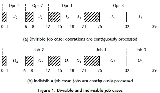
Before we proceed with our analysis, it seems appropriate to illustrate the problem with a numerical example.

Example 1. Consider a simple instance of the problem in which there are three indivisible jobs and four different types of operations. Job 1 has operations 1 and 3; Job 2 has operations 1, 2, and 4; and Job 3 has only operation 3. Within the context of customer order scheduling, these three jobs and four operations correspond with three customer orders and four different products ordered by the customers respectively. Setup and processing time (s_k; p_k) for operations 1 to 4 are (3;3), (2;4), (4;7), and (1;5) respectively. As illustrated in Figure 1(a), a feasible schedule for the operation families is O₄(J₂)-O₂(J₂)-O₁(J₂ - J₁) -O₃(J₁ - J₃)in the traditional single-machine scheduling problem with multi-operation jobs. However, a feasible schedule of the jobs in our problem is J₂(O₄ -O₂ -O₁)- J₁(O₁ -O₃)- J₃(O₃), as illustrated in Figure 1(b). Note that there is no need for a setup for operation 1 in Job 1 since the last operation of the previous job (Job 2) is operation 1; and there is no need for a setup for operation 3 in Job 3 since the last operation of the previous job (Job 1) is operation 3. In both of the feasible schedules in Figures 1 (a) and 1 (b), the makespan is 39, and the total completion time of the jobs is 18 + 32 + 39 = 89. It is clear that the makespan (or total completion time) values in the divisible and indivisible cases may not be the same for every problem instance.

 

 

3.2 Some observations and structural properties of the optimal schedules

Property 1. For both makespan and total completion time minimisation problems, there exists an optimal schedule without inserted idle time.

Proof. If an idle time exists on the machine, then shifting the subsequent jobs left - along with their operations - is feasible, since there are no precedence relationships among the jobs, and this left shifting does not increase the objective value of the current schedule.

Although Property 1 is intuitively obvious, we provide its proof for the sake of completeness.

The set of jobs J can be divided into two disjoint sets J' and J", where the set J' is composed of jobs having no common operation with other jobs, and its complement set J" is composed of remaining jobs, such that J = J' υ J" and J' Ո J" = 0.

The following polynomial-time algorithm decomposes job set J into job sets J and J .

Step 1: Form an N by K matrix where the rows and columns represent the jobs and operations respectively. Set each entry in this matrix to 1 if the job J_jhas operation O_k. Set operation index, k=1.

Step 2: Repeat until (k=K).

(a) Calculate the number of jobs having operation Ok.

(b) If total number of jobs having operation Ok is greater than two, then put all jobs having operation o into the job set J"; otherwise, set k=k+1.

Step 3: Put all remaining jobs in set J into J .

Property 2. There exists at least one optimal schedule of the makespan minimisation problem in which the jobs in set J are not intermingled with the jobs in set J . That is, the jobs in set J are processed successively in any order before or after the optimal sequence of the jobs in set J

Proof. Suppose that J_jis a job in set J . Furthermore, suppose that J_land J_mare two jobs in set J". It is obvious that processing the job Jj between J_land J_mmay prevent the earlier completion of the job J_mif the jobs J_land J_mhave a common operation that may reduce the makespan. Thus the job J_jin set J should not be intermingled with the jobs in set J .

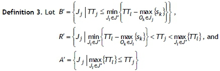
Definition 1. Total time (TT_j) of a job J_jis the sum of the setup and processing times of all jobs in this group - i.e., TTj =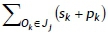

Definition 2. The shortest total time (STT) sequence is a sequence (denoted by σ_STT) in which the jobs are sequenced in non-decreasing order of their total time.

When the setup times are omitted, we observe that the problem reduces to the scheduling of N jobs, with several common and uncommon operations forming a single operation in each job, since all operations of a job are being processed contiguously. In this reduced problem, the makespan minimisation becomes trivial, since any sequence of jobs gives the same objective value. On the other hand, processing the jobs in STT sequence minimises the total completion time of the jobs, where the total time of a job is only the sum of the processing times of the operations in this job, since the setup times are omitted. However, the structure of the problem changes dramatically when the setup times are introduced. Depending on the composition of the jobs, the total completion time minimisation problem is not straightforward, as in the case of no-setup times, and the shortest total time rule does not perform well.

be three disjoint subsets of the set J , which is composed of jobs having no common operation with other jobs.

From Property 1 and Definitions 1 to 3, we have the following result.

Property 3. For the total completion time minimisation problem, there is an optimal schedule with the following properties:

(a) Jobs in subset B precede all other jobs, and jobs in subset A succeed all other jobs.

(b) Jobs in subsets B and A" are scheduled in STT sequence.

That is,

^(J_STT(B") -» {Optimal schedule of J" υ R } -> σ_STT(A')

Proof. Without loss of generality, we assume σ = {/[ψ J_[2],..., J_{[i 1]}, J_[i], J_[i+i],---, J_[n]} is any sequence of all jobs, where J_[j]is the job processed in the j th position of the job sequence σ .

Case A: Suppose that job J_[j]is the first job of type B in the sequence. That is, all jobs preceding the job Jj] are the members of the other sets J", R, and A . Let C_[j]and TC (σ) be the completion time of the job J_[j]in the sequence σ and the total completion time of the sequence σ respectively. Then we have

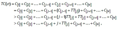
by Definition 3. Moving job J_[j]to the beginning of all jobs in sets J", R, and A currently preceding the job J_[j]in the job sequence σ , and shifting backward all these jobs in sets J", R, and A currently preceding the job J_[j], yields a new job sequence σ = [J_[J],J_[1],J_[2],...,J_[J-i],J_[J+i],---;J_[n]}· Let ΤC(σ') be the total completion time of the job sequence σ'. Then we have

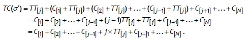
Thus it is clear that the total completion time of the current sequence σ is improved by this change, since ΤC(σ) > ΤC(σ'). Repetition of this argument for all remaining jobs in subset B shows that jobs of the subset B precede all other jobs.

Case B: Suppose that the job J_[j]is the last job of type A in the sequence σ . That is, all jobs succeeding the job J_[j]are the members of the other sets B', J", and R . Then, we have

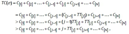
by Definition 3. Moving job J_[j]to the end of all the jobs in sets B , J", and R currently succeeding the job J_[j]in the job sequence σ , and shifting forward all these jobs in the sets B , J", and R currently succeeding the job J_[j], yields a new job sequence

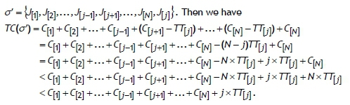
Thus it is clear that the total completion time of the current job sequence σ is improved by this change, since ΤC(σ) > ΤC(σ'). Repetition of this argument for all remaining jobs in the subset A shows that jobs of the subset A succeed all other jobs.

The proof of the second property follows from the result by Smith [25], who showed that processing the jobs in the shortest processing time (SPT) rule minimises the total completion time for the classical single-machine problem in which there are N jobs. In our problem, it is clear that the jobs in the subsets A and B may each be treated as pseudo-jobs in the classical single-machine problem, yielding an optimal sequence characterised by a modified version of SPT, which we refer to as the STT sequence, in which the jobs in the subsets A and B are sequenced in non-decreasing order of their total time TTj. This completes the proof.

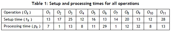
Example 2. Consider an instance of the total completion time minimisation problem in which there are seven indivisible jobs. Setup and processing times for all operations, and the operations in each job, are given in Tables 1 and 2 respectively.

 

 

 

 

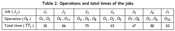
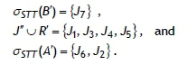
The set of all jobs can be divided into two disjoint sets J' and J", where the set J' = {J₂, J₆, J₇} is composed of jobs having no common operation with other jobs, and its complement set J" = {J_1;J₃,J₄,J₅} is composed of the remaining jobs. From Property 3, the set J' = {J₂,J₆,J₇} decomposes into three subsets: B = {J₇}, A = {J₂, J₆}, and R = 0 since TT₇ = 20 < 21, where

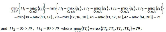
From Property 3, we obtain

The optimal schedule in set J" u R = {J_1; J₃, J₄, J₅} is obtained by solving the MILP model described in Section 5.1, and illustrated in Table 3.

 

 

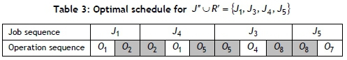
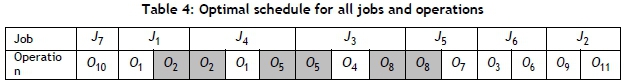
From Property 3, and the MILP model giving the optimal schedule for J" u R, we obtain the following resulting optimal schedule of all jobs and operations (Table 4).

 

 

4 THE MAKESPAN PROBLEM

In this section, we describe the shortest path formulation for the makespan minimisation problem by constructing a network, and show that the problem can be solved in polynomial time. It is clear that the application of Property 2 given in Section 3 will reduce the size of the problem by dropping the jobs in set J from the problem before applying the shortest path network approach to the groups in set J .

4.1 Shortest path network

The shortest path network for minimising the makespan problem consists of a set of nodes and a set of arcs connecting certain pairs of the nodes, as shown in Figure 2, for the numerical example in Section 1. In this Figure, sample feasible and infeasible paths (job sequences) are illustrated. The path passing through the nodes (1, J₂,O₁), (2, J₁,O₁) and (3, J₃,O₃) is a feasible path (job sequence), since jobs J₂, J₁, and J₃ are processed in positions 1, 2, and 3 respectively. However, the path passing through the nodes (1, J₂,O₄ ), (2, J₃,O₃ ), and (3, J₂,O₂ ) is an infeasible path and should be prevented, since job J₂is processed in both positions 1 and 3.

 

 

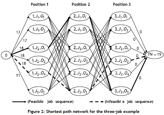
The node set in the network includes:

• A dummy beginning (source) node (0).

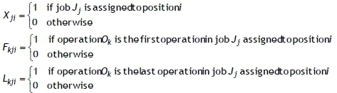
• Intermediate nodes (i, J_j,O_k), i = 1,...,N , j = 1,...,N, k = 1,...,K, \/O_k e Jj : each of these types of nodes represents that job Jj is assigned to the i th position of the job sequence, and operation O_kin job J_jis assigned to the last position in the operation sequence of this job. For each position in the job sequence, which corresponds to a stage in the shortest path network, we created nodes, where NO is the total number of operations in all jobs, and n_jis the number of operations in job J_j. Thus the total number of intermediate nodes is N χ NO.

• A dummy ending (sink) node (TN = N χ NO +1).

The directed arc set A is generated as follows:

• An arc from the beginning node (0) to node (1, Jj,O_r), with flow cost

• An arc from node (i,Jj,O_c) to node (i +1,J_l,O_c), with flow cost , where i = 1,...,N-1, j ≠ l, and O_cis a common operation in jobs Jj and J_l.

• An arc from node (i,Jj,O_r) to node (i +1,J_l,O_v), with flow cost where i = 1,...,N -1, j ≠ l, r ≠ v.

• An arc from node (N, Jj,O_k) to the ending node (TN), with flow cost of zero.

• All the remaining arcs with a flow cost of infinity (or a sufficiently large positive number).

The arcs having a flow cost of infinity are not shown in the network given in Figure 2. This is done to reduce the visual complexity of the network. Thus the network in Figure 2 can be assumed to be incomplete. For example, the arcs between nodes (1, J₁,O₁) and (2, J₁,O₁) and the arc between nodes (1, J₁,O₁ ) and (2, J_1;O₃) are not illustrated in the network, since job J₁ cannot be processed in both positions 1 and 2 of the job sequence. Similarly, the arcs between nodes ( 1,J₁,O₃) and ( 2, J₁,O₁) and the arc between nodes (1, J₁,O₃ ) and (2, J_1;O₃) are also not illustrated in the network, since job J₁cannot be processed in both positions 1 and 2.

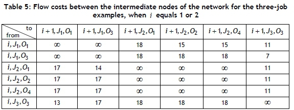
The flow costs between the intermediate nodes of the network for the numerical example in Section 1 are given in Table 5.

 

 

4.2 Mathematical model

The following binary integer programming (BIP) model needs to be solved to find the shortest path in the network.

Parameters, indices, and sets:

TN Number of nodes in the network

f ,t Indices for nodes (f = 0,1,...,TN ; t = 1,2,...,TN )

N Number of jobs

j Index for jobs (j = 1,2,...,N )

cf_t Cost of flow from node f to node t (i.e., on arc (f,t) e A )

h_j,t 1 if node t has job J_j; 0, otherwise

Decision variables:

xf_ttFlow on the arc (f, t) e A

BIP model:

subject to:

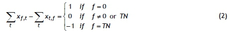
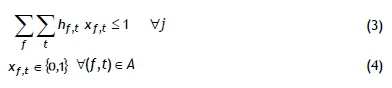
In the model above, the objective in (1) is to minimise the total cost of flow from the source node to the sink node. Constraint set (2) is the conservation equation at each node. Constraint set (3) guarantees that each job is assigned to one position only. Constraint set (4) imposes an integrality restriction on the decision variables.

The BIP model above, excluding the additional side constraints in (3), is a well-known formulation for the classical shortest path problem that can be solved in polynomial-time using the Dijkstra algorithm. However, this solution may not provide an optimal solution that satisfies the additional side constraints in (3), so the BIP model above should be considered for our modified shortest-path problem with constraints in (3). It is clear that the existence of the constraint set (3) prevents the infeasible job sequence. Furthermore, it is known that the node-arc incidence matrix associated with the conservation equations in (2) above is totally unimodular. At least one optimal solution to the linear programming (LP) relaxation of the model above thus exists, in which all decision variables are integer - i.e., x_f,t = 0 or 1. Such a solution can be found by replacing x_f,_t e {0,1} by x_f,_t > 0 and solving the resulting LP. Thus the makespan problem can be solved in polynomial time.

 

5 THE TOTAL COMPLETION TIME PROBLEM

In this section, we present a mixed integer linear programming (MILP) model to solve the total completion time minimisation problem.

5.1 Mathematical model

The following indices, sets, parameters, and variables are used to develop our model.

Parameters, indices, and sets:

N Number of jobs

j Index for jobs (j = 1,2,...,N )

K Number of operation types

k Index for operation types (k = 1,2,..., K)

i Position index for jobs in the sequence (i = 1,2,..., N)

D_jk 1 if job Jj has operation O_k; otherwise, 0

p_k Processing time for operation O_k

s_k Setup time for operation O_k

K_j Set of distinct operations in job J_j

M Set of jobs having more than one operation to be performed

TTj Total (setup and operations) time of job Jj, where TTj =

ST_hkSetup time between operations O_hand O_kis equal to s_k(k ≠ h ) if operation O_k immediately follows operation O_h; otherwise, 0

Decision variables:

RT_Ji = Realized total(setupand operations time of job Jj assignedto positioni

TC = Total completion time of the jobs

MILP model:

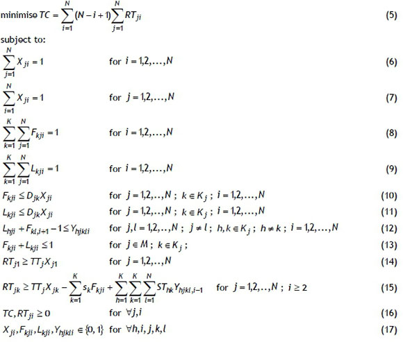
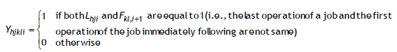
In the MILP model above, the objective in (5) is to minimise the total completion time. Constraint sets (6) and (7) ensure that each position in the job sequence is occupied by one job only and that each job is assigned to one position only, respectively. Constraint sets (8) and (9) guarantee that only one operation in each job can be performed as the first or last operation in its job respectively. Constraint sets (10) and (11) ensure that an operation cannot be the first or last operation of a job, if this job does not include this operation. Constraint set (12) satisfies the condition that no setup time is necessary before the first operation of a job, if this first operation is the same as the last operation of the immediately preceding job. Constraint set (13) guarantees that each operation in a job can be the first, immediate, or last operation of this job. Constraint sets (14) and (15) define the realised total (setup and operations) time of the jobs assigned to the first and other positions respectively. Constraint sets (16) and (17) impose non-negativity and binary restrictions respectively on the decision variables.

5.2 Lower and upper bounds of the total completion time

To improve the efficiency of the MILP model, we introduce a lower bound on the total completion time value. A lower bound LB can be calculated by assuming that:

• the operation with the longest setup time in each job is assigned to the first position of its job,

• the setup time of the operation with the longest setup time in each job is cancelled, by assuming that this operation is the same as the one in the last position of the previous job, and

• all jobs are sequenced in non-decreasing order of their revised total time

Instead of assuming an initial upper bound on the total completion time as infinity, the total completion time value obtained by sequencing all jobs in non-decreasing order of their total time TTj can be used as an upper bound UB . Let TT_STT[i]be the total time of the job in the i th position of the job sequence, in which jobs are sequenced in non-decreasing order of their total time (i.e., shortest total time rule). Then the total completion time becomes the upper bound - i.e., 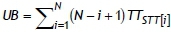. Finally, we add the constraints LB< TC and TC < UB to the mathematical model.

In the MILP model, including the lower and upper bounds on the total completion time, one set of the decision variables is a continuous variable, and the other N² χ [1 + NO χ (N + 2)] of the decision variables, where , is the 0-1 type. On the other hand, the MILP model has 4N + N² χ [1 + |M| + NO χ (NO χ (N -1) - N +1)]+ 2 constraints.

5.3 Computational experiments

In this section, we describe our computational tests to evaluate the effectiveness and efficiency of the MILP model in finding the optimal schedules. The mathematical model is solved by using CPLEX 11.0 in GAMS 22.6, and all computational experiments are conducted on a personal computer with Intel Core i7 dual-core 2.20 GHz CPU and 4 GB RAM. In our experiments, we limit the runtime of the CPLEX to obtain the optimal solution of each problem instance to 10,800 seconds (3 hours).

The solver CPLEX gives two types of solutions for the MILP models. One of the solutions is the best integer solution, which is the desired one; the other solution is the best non-integer solution, in which some of the variables are non-integer. If the best non-integer solution obtained is equal to the best integer solution, then we conclude that the optimal solution is achieved by the MILP model.

5.3.1 Computational settings for test problems

The values of the parameters used in our experiments are generated as follows:

Number of jobs (N): We consider four different cases in which the number of jobs is 5, 10, 15, and 20 respectively.

Number of operation types (K): We consider four different cases in which the number of operation types is 5, 10, 15, and 20 respectively.

Number of operations within each job: We consider two different cases in which the number of operations within every job is variable (changes from one job to another) and constant (same for all jobs). The number of operations is generated from the following discrete uniform distributions:

VARIABLE: DU[1, K]; CONSTANT: DU[2, K-1]

Processing times: We investigate two different cases of the processing times: short and long. They are generated from the following discrete uniform distributions:

SHORT: DU[1, 10]; LONG: DU[100, 200]

Setup times: We investigate four different cases of the setup times. They are generated from the following discrete uniform distributions:

LOW mean - LOW variance: DU[25, 35]; LOW mean - HIGH variance: DU[10, 50]

HIGH mean - LOW variance: DU[55, 65]; HIGH mean - HIGH variance: DU[40, 80]

For each possible combination of the above parameters, five problem instances are generated. Hence a total of 1280 problems are tested.

5.3.2 Discussion of the results

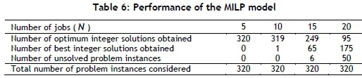
In this section, the performance of our MILP model is discussed. Table 6 shows a summary of the number of problem instances solved optimally within the pre-set time limit (3 hours). As shown in Table 6, all problem instances can be solved optimally when the number of jobs is five. It is clear that the number of unsolved problem instances increases when the number of jobs increases. This shows that the number of jobs causes an increase in the computational time required to solve the problem of optimality.

 

 

To emphasise the performance of the MILP model, we should investigate the quality of the solutions that are not optimal. It is a common phenomenon that the MILP model ends up with a gap between the solution found and the best possible solution. Gap values are therefore examined to indicate the percentage difference in integer solution from the theoretical optimum. We analysed gap values for 241 non-optimally solved problem instances under three circumstances: best case, worst case, and average case. For some of the problem instances, so many iterations were done, and the integer solutions were found to come closer to the theoretical optimum after each iteration. However, CPLEX was terminated because of the time limitation before reaching the optimum solution. But this case was the best case as, when the three-hour time limitation was complete, the gap values were very close to zero. In the worst case analysis, we focused on the problem instances whose solution procedure (branching) was terminated due to memory errors that occurred after a few iterations had been completed. In this case, the integer solutions that are found are very rare, and so the gap values are high. The maximum gap value, which represents the worst case, was found to be 22.92 per cent. On the other hand, branching becomes very difficult for some problem instances, and time-consuming. When branching is slow, the number of iterations is moderate - which leads to higher gap values than the best case, and lower gap values than the worst case. In the average case analysis, the gap values were found to be 0.56 per cent on average.

We also investigated the effect of the lower and upper bounds - given in Section 5.2 - and that are considered constraints in our MILP, on the computational time effort of the solver CPLEX. In our experiments, we observed that the average percentage of reductions in the computational time were 55.6, 30.3, 37.1, and 25.6 for problem instances solved with 5, 10, 15, and 20 jobs respectively, when we used the lower and upper bounds in our MILP. On the other hand, the average percent reductions in the computational time were 43.1, 33.6, 37.7, and 34.1 for problem instances solved with 5, 10, 15, and 20 operations respectively. As seen from these results, it is not possible to observe a significant change in the direction of the computational time while the number of jobs or number of operations increases. However, the greatest reduction in the computational time is seen in small size problems. Considering all problems solved, we observed that the inclusion of the lower and upper bounds in the MILP significantly reduced (by about 37% on average) the computational time.

 

6 CONCLUSIONS AND FUTURE RESEARCH DIRECTIONS

In this study, a relatively new variant of the single-machine scheduling problem of multi-operation jobs with setup times is considered. It is assumed that all operations in a job are processed contiguously, rather than being intermingled with the operations from different jobs (i.e., jobs are indivisible); and no setup time is necessary before the processing of the first operation of a job if this first operation is the same as the last operation of the immediately preceding job. We have investigated the problem with two objectives: one is to minimise the makespan, and the other is to minimise the total completion time of jobs. For the makespan problem, we have shown that the problem is solvable in polynomial time. For the total completion time problem, we have developed a mathematical programming model that obtains optimal solutions for small and medium-sized problems, and near-optimal solutions for large-sized problems. From our experiments it is observed that solving the problem with a standard MILP solver seems not to be a useful alternative, especially for instances of large-sized problems.

A considerable number of issues remain open for future research. Several extensions of our study can be investigated. Although the MILP model was able to solve the small and medium-sized problem instances considered in this paper, and obtained a very small gap between the solution found and the best possible solution for the unsolved large-sized problem instances, future work could develop heuristic algorithms to solve the large-sized problem instances with the objective of minimising the total completion time. Studying different problem characteristics - such as ready times, precedence relations among the jobs, and performance measures (such as total tardiness, maximum lateness, and number of tardy jobs) - would be possible extensions. More complex machining environments with parallel machines or multiple stages could be other future research issues.

 

REFERENCES

[1] Baker, K.R. 1974. Introduction to sequencing and scheduling. New York: Wiley.         [ Links ]

[2] Allahverdi, A. & Soroush, H.M. 2008. The significance of reducing setup times/setup costs. European Journal of Operational Research, 187(3), pp. 978-984. URL: https://www.sciencedirect.com/science/article/pii/S0377221706008162        [ Links ]

[3] Schuurman, J. & van Vuuren, J.H. 2016. Scheduling sequence-dependent colour printing jobs. South African Journal of Industrial Engineering, 27(2), pp. 43-59. URL: http://sajie.journals.ac.za/pub/article/view/1119/683        [ Links ]

[4] Gupta, J.N.D., Ho, J.C. & van der Veen, J.A. 1997. Single machine hierarchical scheduling with customer orders and multiple job classes. Annals of Operations Research, 70, pp. 127-143. URL: https://link.springer.com/article/10.1023/A%3A1018913902852        [ Links ]

[5] Gerodimos, A., Glass, C., Potts, C.N. & Tautenhahn, T. 1999. Scheduling multi-operation jobs on a single machine. Annals of Operations Research, 92, pp. 87-105. URL: https://link.springer.com/article/10.1023/A%3A1018959420252        [ Links ]

[6] Yang, D.L., Hou, Y.T. & Kuo, W.H. 2017. A note on a single-machine lot scheduling problem with indivisible orders. Computers â Operations Research, 79, pp. 34-38. URL: http://www.sciencedirect.com/science/article/pii/S0305054816302520        [ Links ]

[7] Julien, F.M. & Magazine, M.J. 1990. Scheduling customer orders: An alternative production scheduling approach. Journal of Manufacturing and Operations Management, 3(3), pp. 177-99.         [ Links ]

[8] Ahmadi, R.H. & Bagchi, U. 1993. Coordinated scheduling of customer orders. Working paper, John E. Anderson Graduate School of Management, University of California, Los Angeles.         [ Links ]

[9] Gupta, J.N.D. 1984. Optimal schedules for single facility with two job classes. Computers & Operations Research, 11(1), pp. 409-413. URL: https://www.sciencedirect.com/science/article/pii/030505488490042X        [ Links ]

[10] Gupta, J.N.D. 1988. Single facility scheduling with multiple job classes. European Journal of Operational Research, 33(1), pp. 42-45. URL: http://www.sciencedirect.com/science/article/pii/0377221788902524        [ Links ]

[11] Baker, K.R. 1988. Scheduling the production of components at a common facility. IIE Transactions, 20(1), pp. 32-35. URL: http://www.tandfonline.com/doi/abs/10.1080/07408178808966147        [ Links ]

[12] Coffman, E.G., Nozari, A. & Yannakakis, M. 1989. Optimal scheduling of products with two subassamblies on a single machine. Operations Research, 37(3), pp. 426-436. URL: http://pubsonline.informs.org/doi/abs/10.1287/opre.37.3.426        [ Links ]

[13] Aneja, Y.P. & Singh, N. 1990. Scheduling production of common components at a single facility. IIE Transactions, 22(3), pp. 234-237. URL: http://www.tandfonline.com/doi/abs/10.1080/07408179008964178        [ Links ]

[14] Ding, F.Y. 1990. A pairwise interchange solution procedure for a scheduling problem with production of components at a single facility. Computers â Industrial Engineering, 18(3), pp. 325-331. URL: http://www.sciencedirect.com/science/article/pii/036083529090054P        [ Links ]

[15] Mason, A.J. & Anderson, E.J. 1991. Minimizing flow times on a single machine with job classes and setup times. Naval Research Logistics, 38(3), pp. 333-350. URL: http://onlinelibrary-wiley-com/doi/10-1002/1520-6750(199106)38:3%3C333::AID-NAV3220380305%3E3.0.CO;2-0/full        [ Links ]

[16] Potts, C.N. 1991. Scheduling two job classes on a single machine. Computers & Operations Research, 18(5), pp. 411-415. URL: http://www.sciencedirect.com/science/article/pii/030505489190018M        [ Links ]

[17] Liao, C.J. 1996. Optimal scheduling of products with common and unique components. International Journal of Systems Science, 27(4), pp. 361-366. URL: http://www.tandfonline.com/doi/abs/10.1080/00207729608929225        [ Links ]

[18] Gerodimos, A., Glass, C. & Potts, C.N. 2000. Scheduling the production of two-component jobs on a single machine. European Journal of Operational Research, 120(2), pp. 250-259. URL: http://www.sciencedirect.com/science/article/pii/S037722179900154X        [ Links ]

[19] Yang, W.H. 2004. Optimal scheduling of two-component products on a single facility. International Journal of Systems Science, 35(1), pp. 49-53. URL: http://www.tandfonline.com/doi/full/10.1080/00207720310001657072        [ Links ]

[20] Ng, C.T., Cheng, T.C.E. & Yuan, J.J. 2002. Strong NP-hardness of the single machine multi-operation jobs total completion time scheduling problem. Information Processing Letters, 82(4), pp. 187-191. URL: http://www.sciencedirect.com/science/article/pii/S0020019001002745        [ Links ]

[21] Su, L.H. & Chen, Y.H. 2009. Scheduling multioperation jobs on a single flexible machine. International Journal of Advanced Manufacturing Technology, 42, pp. 1165-1174. URL: https://link.springer.com/article/10.1007/s00170-008-1666-3        [ Links ]

[22] Erel, E. & Ghosh, J.B. 2007. Customer order scheduling on a single machine with setup times: Complexity and algorithms. Applied Mathematics and Computation, 185(1), pp. 11-18. URL: http://www.sciencedirect.com/science/article/pii/S0096300306007983        [ Links ]

[23] Hazir, O., Gunalay, Y. & Erel, E. 2008. Customer order scheduling problem: A comparative metaheuristics study. International Journal of Advanced Manufacturing Technology, 3(5-6), pp. 589-598. URL: https://link.springer.com/article/10.1007/s00170-007-0998-8        [ Links ]

[24] Hou, Y.T., Yang, D.L. & Kuo, W.H. 2014. Lot scheduling on a single machine. Information Processing Letters, 114(12), pp. 718-722. URL: http://www.sciencedirect.com/science/article/pii/S0020019014001306        [ Links ]

[25] Smith, W.E. 1956. Various optimizers for single stage production. Naval Research Logistics Quarterly, 3(1), pp. 59-66. URL: http://onlinelibrary.wiley.com/doi/10.1002/nav.3800030106/full        [ Links ]

 

 

Submitted by authors 7 Jul 2018
Accepted for publication 18 Apr 2019
Available online 29 May 2019

 

 

* Corresponding author. cetinkaya@cankaya.edu.tr