GENERAL ARTICLE

 

Improvements towards the identification and quantification of relationships between key performance indicators

 

 

J.L. Jooste^*; L.J. Botha

Department of Industrial Engineering, Stellenbosch University, South Africa

 

 

---

ABSTRACT

The quantitative relationships at the performance measurement system (QRPMS) is a methodology for identifying and quantifying relationships between key performance indicators. These relationships present additional information for decision-making purposes. QRPMS employs the Guttman-Kaiser criterion (K1) to complete a critical step during the methodology. This study presents evidence that the K1 criterion has limitations that compromise the reliability of QRPMS's results. An improved QRPMS version is developed, and the results of the existing and improved QRPMS are compared in a mining industry case study. It is shown that the improved QRPMS delivers more accurate and reliable results.

---

OPSOMMING

Die quantitative relationships at the performance measurement system (QRPMS) is 'n metodiek om verwantskappe tussen sleutel prestasie-aanwysers te identifiseer en te kwantifiseer. Hierdie verwantskappe bied addisionele inligting vir besluitnemingsdoeleindes. QRPMS maak gebruik van die Guttman-Kaiser kriterium (K1) vir die uitvoering van 'n kritieke stap gedurende die metodiek. Die studie lewer bewys dat die K1 kriterium beperkinge het, wat die betroubaarheid van QRPMS resultate beïnvloed. 'n Verbeterde QRPMS weergawe word ontwikkel, en die resultate van die bestaande en verbeterde QRPMS word vergelyk in 'n mynbou-industrie gevallestudie. Die meer akkurate en betroubare resultate van die verbeterde QRPMS word geïllustreer.

---

 

 

1 INTRODUCTION

The use of performance measurement systems in industry is extensive. The challenge is that many key performance indicators (KPIs) are defined as part of these systems, but there is limited understanding of how these KPIs impact outcomes and each other. To gain an improved understanding of KPIs is not a trivial task. Each KPI can have multiple attributes of direction, strength, and polarity. For example, improving some KPIs might worsen others, and the impact of a KPI might be delayed and only become apparent at a later stage [1, 2]. To address these challenges, the importance of quantifying inter-relationships between KPIs has been studied. Rodríguez, Saiz and Bas [3] presented initial research on the topic, and later followed it up with their quantitative relationships at the performance measurement system (QRPMS) methodology [4]. More recent work explores KPI inter-relationships in service delivery [1, 2], the manufacturing industry [5], and cellular network systems [6]. With the ease of data collection brought about by technological developments and the significant contribution that inter-KPI relationships may have on organisational decision-making, it is evident that methodologies such as QRPMS are important in managing organisational performance.

Research has previously been conducted into frameworks and methodologies employing the concept of relationships between performance elements to achieve their respective objectives [7, 8, 9]. These frameworks are, however, limited in their ability objectively to identify and quantify inter-KPI relationships. The reasons for these limitations lie in basic flaws and shortcomings in the two analysis techniques - subjective analysis and pair-wise correlation analysis - used by these frameworks. Subjective analysis is problematic since it is easily influenced by the biased opinions of analysts. It can therefore not be considered a mathematically accurate and reliable analysis technique. Any introduction of subjective analysis into the computational elements of a framework compromises the mathematical validity of the results, and thus any claims of objective results [3].

According to pair-wise correlation analysis, inter-KPI relationships are categorised into three groups: parallel, sequential, and coupled relationships [10]. Investigation into pair-wise correlation shows that it only considers the strong cause-effect relationship between two KPIs [10]. Other influences may be caused by third-party KPIs that may have changing effects on the relationship between the first and second KPIs. This problem is magnified when such a pair-wise correlation analysis technique is employed to identify relationships between a large set of KPIs. It is for this reason that pair-wise correlation analysis is regarded as an unsuitable technique when the aim is to identify inter-KPI relationships [3]. In response to the limitations identified in the frameworks and methodologies, the QRPMS methodology was developed [3]. QRPMS actively avoids the use of any subjective analytical or pair-wise correlation techniques, and employs two mathematical techniques to complete the objective identification and quantification of inter-KPI relationships. Principal component analysis (PCA) is employed to identify the relationships, and partial least squares (PLS) regression analysis is used to quantify these relationships. These two techniques are considered more objective due to the exclusion of interference bias [3].

Investigation into the constituents of QRPMS identifies an inherent limitation when executing a critical step in the final stages of PCA. PCA is a multivariate statistical technique through which the important information found in a multivariate dataset can be reproduced, with minimal loss of information, by new and fewer variables - referred to as principal components (PCs). PCA computes several PCs that are equal to the total number of variables (KPIs, in this context) being assessed by PCA [11]. The critical step in QRPMS entails the process of selecting the appropriate number of PCs to retain for further analysis, while suffering a minimum loss of information from the original dataset.

The QRPMS methodology employs the Guttman-Kaiser (K1) selection criteria to determine the number of PCs to retain. K1 is, however, not considered to be a reliable or accurate selection criterion, although some publications use it without reservation [12, 13]. This claim is supported by other authors, who agree that K1 cannot be recommended for use in PCA, and should be discarded from the list of acceptable selection criteria [14, 15, 16]. An improved version of QRPMS, in which more accurate and reliable selection criteria are employed, is introduced in this study. This improved methodology is referred to as the quantitative identification of inter-performance measure relationships (QIIPMR) methodology.

The QIIPMR methodology employs two alternative selection criteria to K1: parallel analysis (PA) and the scree plot. These two criteria are selected and included in QIIPMR based on comparison studies [13, 17, 18]. PA is employed by QIIPMR as its primary selection criterion due to its proven mathematical accuracy and reliability. The scree plot is incorporated as a supporting criterion to PA, serving to confirm the PA results and to identify any possible errors.

 

2 METHODOLOGY

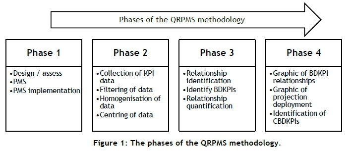
The QRPMS methodology employs four phases to deliver its intended results (Figure 1). The QRPMS phases vary in difficulty, and the time required to complete each may differ depending on the resources available. Phase one consists of the design and analysis of the performance measurement system under consideration. This is followed by the second phase, which covers initial performance measure data treatment. In phase three, the inter-KPI relationships are identified and projected, followed by phase four, which consists of the analysis and presentation of the results.

The QIIPMR is an improved approach to QRPMS: phase three of QRPMS is improved, while the remaining QRPMS phases and processes are incorporated unaltered into QIIPMR. Phase three involves PCA and PLS regression analysis for the identification and quantification of inter-KPI relationships respectively. PCA must be completed to compute the PCs (of the KPI dataset) required for the comparison between QRPMS and QIIPMR. The quantification of the selected PCs (through the execution of PLS) is, however, not performed as part of this paper, for two reasons. First, the quantification of the PCs retained by both methodologies does not contribute additional information to assist in evaluating the improvement offered by QIIPMR over QRPMS. Second, the quantification of KPI relationships using the PLS technique has been successfully validated by previous research, such as that of Patel, Chaussalet and Millard [19] and Rodriguez, Saiz and Bas [3]. To show the improvement of QIIPMR over QRPMS, phases one and two are presented in full, while phase three is partially presented.

 

3 ANALYSIS AND DISCUSSION

Comparing the QRPMS and QIIPMR methodologies appropriately, a set of KPI data from varying organisational sectors - such as operations, engineering, human resources, and logistics - from a single organisation are considered. Such variety of KPI data is not only likely to reveal apparent or obvious inter-KPI relationships, but also relationships between KPIs from different organisational sectors. A case study, in which KPI data from an asset intensive mining organisation is used, serves as a basis for the comparison. The case study organisation consists of different organisational divisions and, most importantly, manages the entire mining and delivery process of a single product, thermal coal. KPI data from a single business entity with sufficient organisational variety is therefore used. This allows a variety of performance data to be available for analysis, presuming that performance measurement and management standards are maintained throughout all organisational divisions. A total of 84 KPIs recorded over two fiscal years are studied. The 84 KPIs consist of those related to the organisation's operations and engineering divisions, safety-related KPIs, KPIs associated with human resources, and KPIs related to the organisation's overall finances. The operations KPIs include KPIs for the sand, dozer, and dragline fleets, drilling units, and the division's overall performance measures. The engineering KPIs include those for the dragline fleet, the shovel, demag crane, excavator, overburden drill, loader, truck, and dozer units.

The multivariate statistics software, Statistica, is used to compute the PCs for the KPI data. Eighty-four PCs are computed in the first exploratory analysis - one for each KPI. Table 1 presents the results of the first 23 PCs. It is important to note from the analysis that, at the 23^rd PC, 100 per cent of the total variance in the KPI data is explained. For the rest of the study, only the first 23 PCs are considered, with the remainder of the PCs being excluded, based on their negligible contribution to the total variance.

 

 

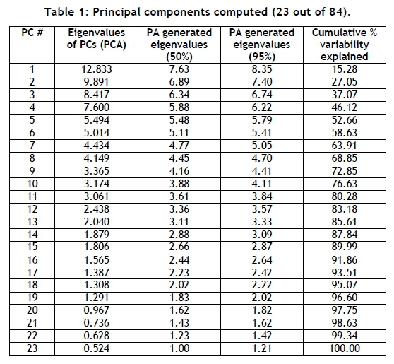
The K1 criterion, used in the QRPMS, states that all PCs with eigenvalues greater than unity may be retained for further analysis. From Table 1, the K1 criterion indicates that the first 19 of the total (84) computed PCs can be retained for further analysis. However, this poses a problem for analysts, since the K1 criterion does not explicitly state which PCs should be retained. Analysts who employ the K1 criterion are required to assess the retainable PCs, and make an informed decision about which of those PCs should be retained. This is the first deficiency of the K1 criterion. This deficiency is addressed in QIIPMR by using PA and the scree plot to identify the specific PCs that should be retained for further analysis. By using Statistica, the PA criterion constituents are calculated, as displayed in Figure 2.

According to the PA criterion, the correct PCs to retain for further analysis are those that have eigenvalues greater than the averaged eigenvalues computed from the random parallel correlation matrices. By consulting Figure 2, it is evident that the first four PCs are extractable, whereas the fifth PC has an eigenvalue barely larger than the mean (50th percentile) eigenvalue, and is thus not extractable.

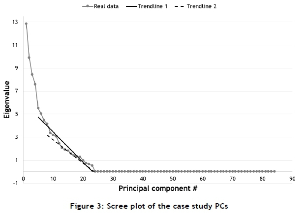
The scree plot requires the PCs to be plotted against their respective eigenvalues, as shown in Figure 3. According to the scree plot, all PCs with eigenvalues that are plotted before a linear decrease are candidates for extraction. However, when consulting Figure 3, it is difficult to ascertain where the appropriate linear decrease starts. To help identify the correct start of an appropriate linear decrease, two linearly decreasing trendlines are included in the plot shown in Figure 3.

The first trendline is fitted to all data points between the fifth PC (the first possible start of a linear decrease) and the 23rd PC (the last, non-zero eigenvalue). The second trendline is fitted to all data points between the eighth PC (the second possible start of a linear decrease) and the 23rd PC. From these two trendlines, the scree plot shows that the first four PCs can be extracted with confidence for further analysis. However, due to the difficulty of determining where the linear decrease starts, the identification of additional PCs (for extraction) cannot be confidently or accurately determined.

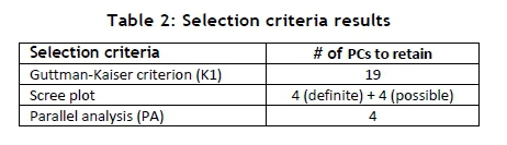
A summary of the three selection criteria and their outcomes is presented in Table 2. To compare the results of the K1 criterion, PA, and the scree plot criteria in detail, it is necessary to investigate the 19 PCs (identified by the K1 criterion) to evaluate their so-called 'retention-value', compared with those PCs identified by PA and the scree plot. A PC is interpreted by assessing the loading coefficients of its contributing variables (KPIs) [20]. Contributing variables with large loading coefficients ('significant' contributing variables, either positive or negative in nature) attach meaning to a PC, whereas variables with small loading coefficients ('insignificant' contributing variables) contribute little meaning.

 

 

In this paper, a PC's retention-value is evaluated by assessing the number of significant contributing variables (KPIs) it contains. PCs are linear combinations of the original KPIs in the data; therefore, a PC with many significant contributing variables is indicative of multiple, strong cause-effect relationships between these 'significant' KPIs. A PC with multiple significant contributing variables therefore has a high retention-value, and is more critical for assessment than a PC with few or no significant contributing variables.

In assessing PCs, analysts are required to decide what magnitude a loading coefficient must exceed for that contributing variable to be classified as a significant contributing variable [21]. There are various methods of determining this magnitude for PC evaluation [21, 22]. Chin [22] suggests that contributing variables with loading coefficients larger than 0.6 (in absolute value) are to be considered significant contributors. To complete the assessment of the PCs shown in Table 1, two values are selected to determine significant contributors: firstly, 0.6, and 0.4 for a more conservative alternative. A sensitivity analysis is performed, comparing the use of these two values.

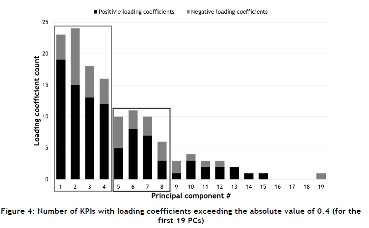
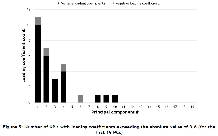
It is important to note that the number of significant contributing variables does not equal the exact number of strong, inter-KPI relationships. Simply identifying the KPIs with significant loading coefficients for each respective PC is not an adequate method for identifying inter-KPI relationships. A matrix containing the loading coefficients of each KPI, for each PC, is computed. From this matrix, the number of contributing variables (KPIs) with loading coefficients exceeding the absolute value of 0.4 (conservative) and 0.6 (recommended) is determined for the first 19 PCs. The results are illustrated in Figure 4 and Figure 5.

From the conservative results (Figure 4), it is seen that the ninth to the 19th PCs have very few significant contributing variables. These PCs are therefore not indicative of many, strong cause-effect relationships between the KPIs in the dataset. The PCs are, however, indicative of some cause-effect relationships between pairs of KPIs. If the retention-values of these PCs are evaluated, based on the number of multiple, strong inter-KPI relationships represented, it is indicative that they have little retention-value or assessment importance compared with the remaining PCs.

Visual assessment of Figure 4 reveals two groups of four PCs with a similar number of significant contributing variables. The first group (PCs 1 to 4) have approximately double the number of significant contributing variables per PC, compared with the second group (PCs 5 to 8). This shows that the first four PCs in Figure 4 contain the largest number of strong inter-KPI relationships of the 19 PCs assessed. This finding is more evident from Figure 5, where only the first four PCs are shown to have more than one significant contributing variable.

From the analysis and comparison, it is concluded that the K1 criterion suggests the retention of multiple 'insignificant' PCs for further analysis. The K1 criterion requires an additional assessment of the results to determine which of the 19 PCs are worth retaining. Based solely on the K1 results, the specific number of PCs that should be extracted could not be determined. The scree plot is more useful than the K1 criterion for showing that the first four PCs should be extracted for further assessment; but it proved difficult to ascertain where the 'cut-off' point is for the extraction of additional potential PCs. However, the PA criterion indicates that the first four PCs should be retained for further analysis.

The study therefore supports the work by Yeomans and Golder [12], Lance and Vandenberg [13], and Zwick and Velicer [14], who also proved that the PA criterion delivers the most accurate and reliable results of the three selection criteria investigated in this case study. The scree plot proved to be an adequate supporting selection criterion for PA, but its sole implementation may prove problematic in assessing the results.

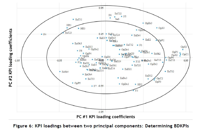
The QRPMS and QIIPMR methodologies both employ a graphical figure to highlight which KPIs are business driver key performance indicators (BDKpIs). Rodriguez et al. [4] state that BDKPIs are of greater importance to organisational management because of the relationships they maintain, and are critical to the evolution of the organisation. Two PCs are plotted against each other (Figure 6), using their respective KPI loading coefficients as data points. Two concentric ellipses are included in the plot. The larger ellipse indicates the 'border maximum', which is the maximum (absolute) value (1.0) that a single loading coefficient can achieve. The second, smaller ellipse indicates the 'border minimum', which is the minimum (absolute) value a loading coefficient must exceed for that variable to be classified as a significant contributor to the PC.

This border minimum is determined by computing the minimum (absolute) value that each of the corresponding KPI loading coefficients (from the two PCs) must exceed for the resulting vector to have a magnitude greater than or equal to unity. The border minimum (absolute) value is computed to be 0.7, a value also used by Rodriguez et al. [4]. Figure 6 depicts the border maximum and border minimum for the first and second PCs computed in the case study for the QIIPMR methodology. The KPIs that fall in the area between the two concentric ellipses are reclassified as BDKPIs; this is repeated until all PCs are plotted against each other. The BDKPI prefix indicates the organisational division that measures the respective BDKPIs. The prefixes are: En for Engineering, F for Finance, HR for Human Resources, Op for Operations, and Sa for Safety.

The BDKPIs identified by QRPMS and QIIPMR are shown in Table 3 and Table 4 respectively. Table 4 contains 26 identified BDKPIs (only using the four PCs identified by PA and the scree plot). Therefore, 26 of the 84 KPIs are of greater importance to organisational management because of their inherent relationships. And a mixture of KPIs from Finance, Operations, Engineering, Safety, and Human Resources constitute those BDKPIs listed in Table 4, satisfying the desire to identify inter-KPI relationships between the mine's focus performance areas.

 

 

 

 

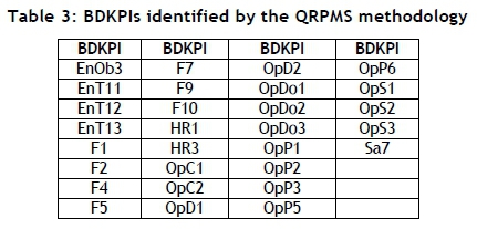
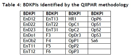
To complete the final comparison between QIIPMR and QRPMS, it is necessary to compare the BDKPI results. QIIPMR and QRPMS identify 26 and 29 BDKPIs respectively. When considering the number of PCs used by each methodology to determine their respective BDKPIs (four PCs versus 19 PCs respectively), it is apparent that the retention of additional, less important PCs (as in the case of QRPMS) yields diminishing returns. Furthermore, there are differences between the BDKPI results listed in Table 3 and those in Table 4. Only 15 BDKPIs correspond between the two sets of results. Table 5 presents the BDKPI comparison results, categorising them against the organisational divisions.

 

 

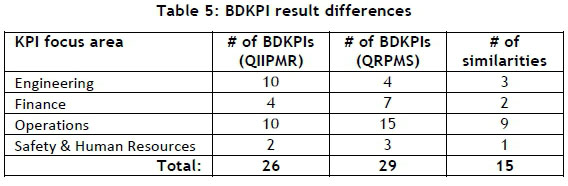
The results in Table 5 show additional noteworthy differences. QIIPMR identifies more than double the number of Engineering BDKPIs than QRPMS, and QRPMS identifies 50 per cent more Operations BDKPIs than QIIPMR. Similar differences are apparent for the Finance and Safety and Human Resources BDKPIs. It is evident from the comparison that it cannot be assumed (when determining BDKPIs in this case study) that employing 19 PCs will result in the identical BDKPIs that the first four PCs will identify.

One possible reason for the variation between the two sets of BDKPIs shown in Table 5 may be the recalculation of the PCs while limiting the total number of PCs (that can be calculated) to four and 19 (for QIIPMR and QRPMS respectively). The recalculated PCs may differ from their KPI loading coefficients. However, this is not the case. The loading coefficients of every KPI, for each PC, remain the same, regardless of the limitation.

Although an exhaustive assessment of the BDKPI differences between QIIPMR and QRPMS was not covered in the study, Yeomans and Golder [12], Zwick and Velicer [14], Velicer, Eaton and Fava [15], and Cortina [16] state that the K1 criterion is highly inaccurate. Their research is indicative that the K1 criterion compromises the reliability and mathematical accuracy of the results obtained from QRPMS, and could explain the different QrPMS and QIIPMR results. Furthermore, the QRPMS results coincide poorly with the results of QIIPMR, which is a similar methodology that uses more accurate and reliable selection criteria. The QIIPMR employs the scree plot as a supporting selection criterion to PA, enabling any calculation errors to be identified. Thus, the results of the QIIPMR methodology are argued to be more trustworthy than those of QRPMS.

 

4 CONCLUSION

Quantifying the relationship of many KPIs, and its impact on business outcomes, remains a challenge. The QRPMS methodology provides a basis for quantifying KPI relationships, but has a limitation in the Guttman-Kaiser, or K1, criterion for selecting principal components. It is suggested that the K1 criterion compromises the reliability and mathematical accuracy of the results obtained from QRPMS. This paper presents a study of an alternative approach in the form of QIIPMR, which improves on the QRPMS methodology. QIIPMR makes use of parallel analysis, supported by the scree plot for selection criteria, as an alternative to the K1 criterion. QIIPMR thus simplifies the identification of principal components to prevent statistical errors. The benefits of QIIPMR over QRPMS are illustrated by a case study in the asset intensive mining industry.

 

REFERENCES

[1] Shrinivasan, Y.B., Dasgupta, G.B., Desai, N. & Nallacherry, J. 2012. A method for assessing influence relationships among KPIs of service systems. In: Liu, C., Ludwig, H., Toumani, F. & Yu, Q. (eds), ICSOC 2012. LNCS, Vol. 7636, pp. 191-205. Heidelberg: Springer.         [ Links ]

[2] Dasgupta, G.B., Shrinivasan, Y., Nayak, T.K., Nallacherry, J., Basu, S., Pautasso, C., Zhang, L. & Fu, X. (eds). 2013. Optimal strategy for proactive service delivery management using inter-KPI influence relationships service-oriented computing. Proceedings of the 11th International Conference, ICSOC 2013, pp. 131-145. Berlin Heidelberg: Springer.         [ Links ]

[3] Rodríguez, R.R., Saiz, J.J.A. & Bas, A.O. 2006. Relationships among key performance indicators within the performance measurement system context: Literature review. In: Performance Measurement and Management Conference, London, July 2006, pp. 689-701.         [ Links ]

[4] Rodriguez, R.R., Saiz, J.J.A. & Bas, A.O. 2009. Quantitative relationships between key performance indicators for supporting decision-making processes. Computers in Industry, 60(2), pp. 104-113.         [ Links ]

[5] Kang, N., Zhao, C., Li, J. & Horst, J.A. 2015. Analysis of key operation performance data in manufacturing systems. IEEE International Conference on Big Data, Santa Clara, CA, 2015, pp. 2767-2770.         [ Links ]

[6] Guo, X., Yu, P., Li, W. and Qiu, X. 2016. Clustering-based KPI data association analysis method in cellular networks. In: 2016 IEEE/IFIP Network Operations and Management Symposium, Istanbul, 2016, pp. 11011104.         [ Links ]

[7] Suwignjo, P., Bititci, U.S. & Carrie, A.S. 2000. Quantitative models for performance measurement system. International Journal of Production Economics, 64(1), pp. 231-241.         [ Links ]

[8] [8] Youngblood, A.D. & Collins, T.R. 2003. Addressing balanced scorecard trade-off issues between performance metrics using multi-attribute utility theory. Engineering Management Journal, 15(1), pp. 1118.         [ Links ]

[9] Bauer, K. (2005). KPI reduction the correlation way. Information Management, 15(2), p. 64.         [ Links ]

[10] Cai, J., Liu, X., Xiao, Z. & Liu, J. 2009. Improving supply chain performance management: A systematic approach to analyzing iterative KPI accomplishment. Decision Support Systems, 46(2), pp. 512-521.         [ Links ]

[11] Tabachnick, B.G. & Fidell, L.S. 2001. Using multivariate statistics, 4^th edition, Boston: Allyn & Bacon.         [ Links ]

[12] Yeomans, K.A. & Golder, P.A. 1982. The Guttman-Kaiser criterion as a predictor of the number of common factors. The Statistician, 31, pp. 221 -229.         [ Links ]

[13] Lance, C.E. & Vandenberg, R.J. 2009. Statistical and methodological myths and urban legends: Doctrine, verity and fable in the organizational and social sciences. New York: Taylor & Francis.         [ Links ]

[14] Zwick, W.R. & Velicer, W.F. 1986. Comparison of five rules for determining the number of components to retain. Psychological Bulletin, 99(3), p. 432.         [ Links ]

[15] Velicer, W.F., Eaton, C.A. & Fava, J.L. 2000. Construct explication through factor or component analysis: A review and evaluation of alternative procedures for determining the number of factors or components. In: Goffin, R.D & Helmes, E. (eds), Problems and solutions in human assessment, 2000, pp. 41-71. Boston: Springer.         [ Links ]

[16] Cortina, J.M. 2002. Big things have small beginnings: An assortment of "minor" methodological misunderstandings. Journal of Management, 28(3), pp. 339-362.         [ Links ]

[17] Zwick, W.R. & Velicer, W.F. 1982. Factors influencing four rules for determining the number of components to retain. Multivariate Behavioral Research, 17(2), pp. 253-269.         [ Links ]

[18] Zhu, M. & Ghodsi, A. 2006. Automatic dimensionality selection from the scree plot via the use of profile likelihood. Computational Statistics & Data Analysis, 51(2), pp. 918-930.         [ Links ]

[19] Patel, B., Chaussalet, T. & Millard, P. 2008. Balancing the NHS balanced scorecard! European Journal of Operational Research, 185(3), pp. 905-914.         [ Links ]

[20] Cadima, J. & Jolliffe, I.T. 1995. Loading and correlations in the interpretation of principle components. Journal of Applied Statistics, 22(2), pp. 203-214.         [ Links ]

[21] Dunteman, G.H. 1989. Principal components analysis. Newbury Park, California: Sage.         [ Links ]

[22] Chin, W.W. 1995. Partial least squares is to LISREL as principal components analysis is to common factor analysis. Technology Studies, 2(2), pp. 315-319.         [ Links ]

 

 

Submitted by authors 10 Nov 2017
Accepted for publication 20 Jul 2018
Available online 31 Aug 2018

 

 

* Corresponding author: wyhan@sun.ac.za