GENERAL ARTICLE

 

Management optimisation of mass customisation manufacturing using computational intelligence

 

 

L. Butler; G. Bright^*

Discipline of Mechanical Engineering, School of Engineering, University of Kwa-Zulu Natal, South Africa

 

 

---

ABSTRACT

Computational intelligence paradigms can be used for advanced manufacturing system optimisation. A static simulation model of an advanced manufacturing system was developed in order to simulate a manufacturing system. The purpose of this advanced manufacturing system was to mass-produce a customisable product range at a competitive cost. The aim of this study was to determine whether this new algorithm could produce a better performance than traditional optimisation methods. The algorithm produced a lower cost plan than that for a simulated annealing algorithm, and had a lower impact on the workforce.

---

OPSOMMING

Rekenaarverwerkingintelligensie paradigmas kan gebruik word vir gevorderde vervaardigingstelsel optimering. 'n Statiese simulasie model van 'n gevorderde vervaardigingstelsel is onwikkel. Die doel van die vervaardigingstelsel is om 'n aanpasbare produk op groot skaal te vervaardig teen 'n kompeterende koste. Die doel van hierdie studie is om te bepaal of dié nuwe algoritme 'n beter vertoning as tradisionele optimeringsmetodes lewer. Die algoritme het 'n laer onkoste as die van n gesimuleerde uitgloei-algoritme en het n laer impak op die werksmag gehad.

---

 

 

1 INTRODUCTION

Research in advanced manufacturing systems (AMSs) is striving to achieve mass customisation manufacturing (MCM) [1]. This is driven by the demand from the markets for unique customised products at affordable prices and within reasonable lead times [1]. However, producing customised products at the same cost as high volume, low variety manufacturing has conflicting objectives. Manufacturing researchers have devoted their attention to this problem from different perspectives. Two main research areas - production planning and production scheduling - have been identified as being both fundamental and sufficiently different to focus on separately, in an attempt to improve manufacturing system performance in order to approach full MCM. Computational intelligence (CI) has emerged as a popular instrument to apply in the pursuit of optimising manufacturing systems, both for maximising profitability and for achieving MCM for maximum market share [1][2].

A distinct advantage of the CI paradigm is the techniques involved in producing sets of optimal and near-optimal solutions from which the most acceptable solution can be selected. Decision-makers can still make the final decision. The nature of most CI algorithms makes them robust and adaptable to variations in system parameters and characteristics. For this reason they are well suited to applications in environments based on paradigms that make use of computer-integrated manufacturing (CIM) infrastructure. They are also designed to be flexible. The application of CI optimisation techniques can assist modern manufacturing systems to be more responsive and adaptable to variations in product design due to changing customer demands. This is an important consideration for existing manufacturing enterprises pursuing MCM, and for the purpose of this research study [3][5].

The research methods used in this study relied on the use of simulation modelling for testing and experimentation. A static simulation model of an AMS was created, based on a hypothetical product - a family-based product range designed for MCM. This model was developed using a classical simulation model development process that included verification and validation of the model behaviour. Simulation modelling was used because no real-world system was available for this study.

The aim of this study was to determine whether an algorithm based on a previously unexplored principle could produce a better performance than traditional optimisation methods. Analysis of the results achieved by the implementation of this newly developed optimisation method for the production planning problem was carried out by comparing the two algorithms. An additional optimisation algorithm was written, based on an established artificial intelligence (AI) paradigm found in the literature, in order to measure the performance of the newly developed planning optimisation algorithm.

 

2 MASS CUSTOMISATION FOR ADVANCED MANUFACTURING SYSTEMS

Mass customisation (MC) was first defined by Joseph Pine in 1993 [2] as the production of individually customised goods through the use of flexible and highly responsive advanced manufacturing systems, at a cost near that of mass-produced goods. This is a broad definition that can take many forms at a practical level. In the pursuit of MC, the most popular approaches have been based on delayed product differentiation (DPD), also known as process postponement [3]. Many different implementations of DPD exist. Each is characterised by the point in production at which differentiation occurs; from engineer-to-order, where each instance of the product is designed to the customer's requirements, to package-to-order, where differentiation only occurs at the packaging stage.

In the context of this study, MC was viewed as the differentiation of the product during production; in other words, differentiation is restricted to variants in the product family, and is achieved while the product is in the manufacturing system. This is analogous to the mode of MC described as fixed resource design-to-order MC, according to MacCarthy, Brabazon and Bramham [4]. This selection was made because it is believed that this is the best avenue for modern AMSs to achieve MCM effectively.

2.1 Computational intelligence for mass customisation manufacturing

In the context of this study, the concept of CI was viewed as a development and extension of the concept of artificial intelligence (AI). This may include topics that are regarded as traditional AI, such as artificial neural networks, evolutionary computation, and swarm intelligence [5]. However, in order to avoid limiting the scope of the research to the more established CI/AI paradigms, the definition used here also includes algorithms and methods based on fields such as biology, physics, and chemistry [6].

A literature search analysis carried out in March 2014 showed that 'artificial intelligence' and other keywords relating to this study, such as 'flexible manufacturing systems', started receiving attention in the 1980s, with 10 per cent of all search results coming from that decade. The prevalence climbed steeply from there, with 28 per cent in the 1990s, 35 per cent in the 2000s, and 27 per cent in the 2010s to date. This analysis also produced, on average, eight times more results when using the keywords 'artificial intelligence' rather than 'computational intelligence'. From this it was clear that much more attention has been given to AI in manufacturing systems research than to CI, which is an indication that CI is not quite mature as a field of research in manufacturing systems.

The optimisation of manufacturing systems has been an active field of research, with as many focus areas as there are subsystems. Renzi et al. [7] and Ferreira [8] present exhaustive lists of the literature of CI methods used in optimising AMSs. From the literature it was clear that some of these focus areas have received much attention in research through the application of different methods that can be described as CI, among other methods. The different areas of application have been classified in two broad categories; manufacturing planning and manufacturing operations. These two categories have been used as the basis for this study, with the emphasis on aggregate production planning (APP).

 

3 PRODUCTION SYSTEM MODEL

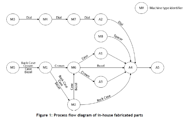
The production system was configured in such a way that, once an in-house fabricated part has been completed, it is transported directly to the workstation where it is required for assembly, instead of using batch transportation. This makes the scheduling of operations more complex, because there are more parts moving around in the system throughout the production run. However, this should be outweighed by the saving in the holding of the finished parts waiting for assembly at separate locations, such as in an automated storage and retrieval system (ASRS). This also forces each part to be fabricated on demand from orders placed by customers, in line with the pull methodology [9]. The process flow of fabricated parts from raw material to final assembly can be seen in Figure 1.

The machine type identifiers in Figure 1 refer to the machine types required to perform the necessary machining operations for the production of men's wrist watches. Similarly, the assembly station identifiers in Figure 1 refer to the assembly workstations required to complete the process of assembling the wrist watches. All raw materials enter the system on the left of the figure, either at M3 or M5 (depending on the part being manufactured), move through the system in a general left-to-right direction, and exit the system as part of a final assembly after assembly station A5. Figure 1 also shows the flow of the major components of the wrist watch through the system.

 

4 PRODUCTION PLANNING OPTIMISATION

Production planning to meet demand forecasts allows a manufacturer to anticipate and plan for variations, which is critical to the success of a manufacturing enterprise. This section presents the development of a novel algorithm to determine an optimal aggregate production plan for a wrist watch product range based on a common product platform. The performance of the new algorithm is compared with traditional planning strategies and with an optimisation algorithm based on a well-established AI principle.

4.1 Biogeography-based optimisation

Biogeography-based optimisation (BBO) is founded on the principle of biogeography, which is the study of species, their migration between habitats, and their extinction [10]. Habitats, also referred to as 'islands', are rated for their fitness to support life, using a term known as the habitat suitability index (HSI). A high HSI is associated with a habitat that is fit to support a large number of species, whereas a habitat with a low HSI is only fit to support a small number of species.

Migration is driven by the number of species within the habitats of the system. This determines the immigration and emigration rates of the species in each habitat, based on a graph similar to that shown in Figure 2 [10]. In other words, a habitat with a high HSI will contain a large number of species, and therefore will have a high emigration rate, μ. In contrast, a habitat with a low HSI will contain a small number of species, and so will have a high immigration rate, λ.

 

 

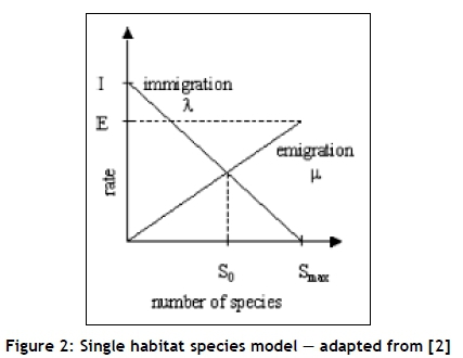
As migration occurs, the increasing species diversity of the low HSI habitats will cause their HSIs to increase, and the reduction in species diversity in the high HSI habitats will cause their HSIs to reduce. This will continue until the number of species reaches an equilibrium, S0. In reality, only a small group of individuals migrate between habitats, leaving a population behind in their original habitat. However, with BBO, entire populations are assumed to migrate. This is necessary because, with BBO, the species represent independent variables of the objective function, which replace each other between the set of candidate solutions, or habitats.

With BBO, λί represents the probability that an independent variable, or species, in the i-th habitat will be replaced [10]. And the probability, P, of a given species in habitat Xj, emigrating from Xj to replace the emigrating species in habitat Xi, is calculated using Equation 1.

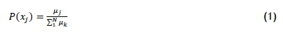
where k = 1, 2, 3, . . . N, and N is the number of habitats in the system. This is based on the principle of fitness proportionate selection, in which selection pressure is proportional to the fitness of the candidates [11].

BBO can also incorporate mutation, which represents the introduction of random disturbances to the HSIs of habitats [10]. The method of deciding whether a given species, or independent variable, in a certain habitat should be mutated is to compare a user-defined mutation probability parameter with a randomly generated number in the same range, and then to mutate the variable by randomly adjusting its value within its range.

4.2 Implementation

The algorithm was based on the work of Simon [10]. The outer loop repeated for a user-defined number of iterations, and the inner loop stepped through the user-defined number of habitats, or candidate solutions. The population of possible solutions - i.e., the aggregate production plans - was generated at the initialisation of the algorithm, based on the production plan parameters. The parameters were calculated based on randomly generated variables: an inventory-to-production ratio, and a workforce level parameter.

The inventory-to-production ratio and workforce level variables were used to vary the inventory-to-production ratio and workforce level from month to month respectively. Equations 2 and 3 show the expressions used for these two variables. The expression for inventory-to-production ratio increased or decreased the ratio of inventory-to-production for each month by up to 17 per cent, while the workforce level variables parameter added up to two workers to, or subtracted up to two workers from, the workforce from one month to the next. These expressions were developed by trial and error, and therefore the numerical constants are specific to the system under investigation.

All the plan parameters were calculated from these two variables. The plan parameters included production levels, workforce levels, and inventory levels for each month in the planning period. In the context of the BBO principle, each plan represented a habitat, and each plan parameter represented a species. The algorithm calculated the cost of each plan, then ranked and sorted them according to their cost. Immigration and emigration rates for each plan were calculated based on the rank of the plan - i.e., the plan with the lowest cost had the highest emigration rate, and the plan with the highest cost had the lowest emigration rate. The immigration rates were calculated by subtracting the emigration rates from 1, as shown in Equation 4.

Iterations began by placing the two lowest cost plans into an elitist matrix for replacing the two highest cost plans in the next iteration. The inner loop then stepped through the habitats, or plans. For each iteration, production plan parameters of each plan were migrated (based on a probability calculated from the HSI), and mutated (based on a predefined probability). The production plan cost was used as the HSI here. The newly migrated and mutated plans were then sorted from lowest cost to highest.

The validity of the lowest cost plan was checked, and if the plan was not valid, that iteration was discarded and repeated with new migrations and mutations. If the lowest cost plan was valid, the algorithm proceeded to store the lowest cost plan of that iteration in a matrix of low cost plans. The validity requirement set, in this instance, was that the ending inventory level in the final month of the planning period be greater than zero.

The algorithm then replaced the two highest cost plans with the two elite plans stored in the previous iteration, and placed the lowest cost plan for that iteration into the low cost plans matrix. The low cost plans matrix held the lowest cost valid plans from each iteration. Once the maximum number of iterations had been completed, the absolute lowest cost valid plan was extracted from the low cost plan matrix for outputting.

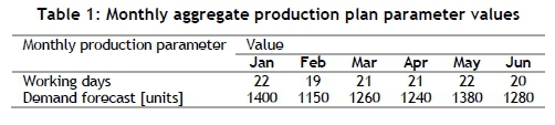
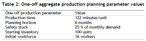
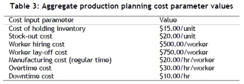
Before the BBO algorithm was initialised, all plan parameters were initialised. Table 1, Table 2, and Table 3 show the plan parameters and the values for which the optimal aggregate production plan was developed.

 

 

 

 

 

 

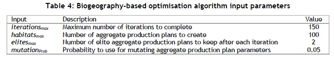
The values of the parameters shown in Table 4 were found through trial and error by comparing the results of the BBO algorithm from subsequent runs of the algorithm. The given values were found to produce the best results within a reasonable search space and time frame. However, because they were found by trial and error, it cannot be categorically stated that this combination of parameters produces the optimal plan.

4.3 Initialisation

Before initialisation of the BBO algorithm, three plans were developed, based on traditional standard planning strategies. These main strategies, according to Chase et al. [3], are:

1. Chase strategy, in which the production rates are matched exactly to the order arrival rate by the hiring and laying off of workers as the order arrival rates vary.

2. Stable workforce - variable work hours, in which production is varied by varying the number of production hours worked, by implementing flexible shifts or overtime.

3. Level strategy, in which the workforce is kept stable, with constant output rates allowing for inventory build-up or shortages.

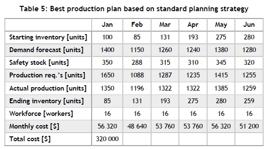
The lowest cost plan from these was used as the starting point for the BBO algorithm, to compare its results. For the problem at hand, the lowest cost plan based on a standard planning strategy was found to be one based on the level workforce / varied production strategy - that is, a stable workforce with varying levels of inventory. Table 5 shows the calculated plan parameters for this plan, including the total cost of production.

 

 

The BBO algorithm programme was written in C++, using Microsoft Visual Studio Express 2013 as a Win32 console application. The solution time for the BBO algorithm was approximately 10 seconds.

 

5 BENCHMARKING USING SIMULATED ANNEALING ALGORITHM

To set a benchmark in order to assess the performance of the new BBO algorithm, a simulated annealing (SA) algorithm was developed and applied to the same case study production system. Simulated annealing was used as a benchmark because it is a well-established AI method, and has been widely used in manufacturing systems optimisation research [7], [12]. The SA algorithm is based on the principle of annealing in metallurgy, where a metal is heated to a high temperature, and then cooled in a slow and controlled manner in order to produce a particular molecular structure in the material [5]. Simulated annealing is a search scheme that incorporates an exploration component and an exploitation component.

The initial state of the system consists of an initial candidate solution that is randomly generated, the system temperature variable T, and the temperature schedule parameter. From the initial state, the neighbourhood of the candidate solution is explored by generating new candidate solutions through varying the solution parameters, based on the current system temperature. This is performed for a certain number of iterations before lowering the system temperature, based on the temperature schedule. At each iteration, the new candidate solution is compared with the best solution found so far, and if the new solution is better, it is stored as the new best solution.

The temperature schedule is a fraction multiplied by the current temperature. The best candidate solution at the current temperature is kept as the starting point for the next round of iterations at the next system temperature. As the system temperature decreases, the search area around the current best candidate solution decreases, which enhances the exploitation component of the search. However, to avoid the search becoming trapped at a local optimum, an acceptance probability is calculated and compared with a randomly generated fraction. Equation 5 shows the expression for calculating the acceptance probability, P.

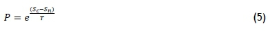
where Sc is the current best solution objective function value, Sn is the newly calculated solution objective function value, and T is the current system temperature [13]. If the acceptance probability is greater than the randomly generated fraction, the new candidate solution replaces the current best candidate solution. This step only takes place if the new candidate solution is not better than the current best candidate solution. In other words, the acceptance probability represents the probability of a worse solution being accepted as a possible optimal solution. However, it can be seen from Equation 5 that the probability tends to zero as the temperature decreases, since the numerator of the exponent will always be negative.

 

6 RESULTS

The results from the new BBO and SA algorithms were compared to measure the performance of the BBO algorithm. This was done from a cost convergence perspective and from the final aggregate production plans produced. All programming was carried out and run on the same computer for consistency.

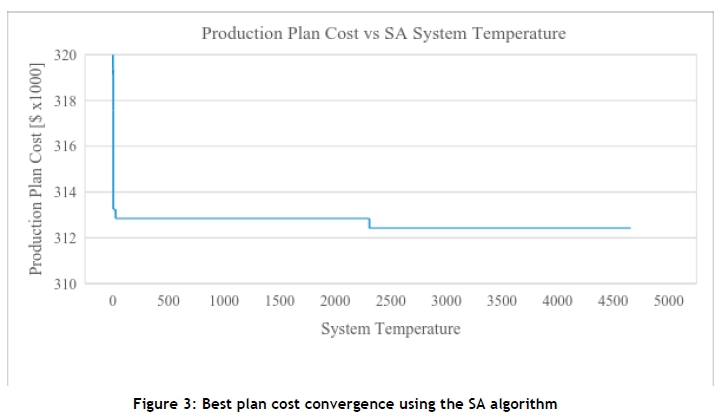
Figure 3 shows the convergence of the overall best plan cost by the SA algorithm, within the first five per cent of the temperature schedule to near-optimal plan, and a final drop to the output value at approximately 50 per cent through the temperature schedule.

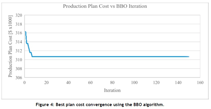
Figure 4 shows the convergence of the lowest plan cost for the BBO algorithm. From this figure it can be seen that the algorithm converged to the final value within the first ten iterations, or approximately seven per cent of the total run length.

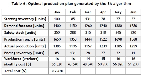
The SA algorithm produced the production plan shown in Table 4.7. This production plan showed an improvement of 2.37 per cent of the total cost compared with the best standard strategy plan. This translated to an average saving of $ 1 263.33 per month, or $ 15 160.00 annually. The SA algorithm produced a plan with lower inventory levels and a relatively small workforce turnover, while tracking the demand forecasts well compared with the best standard strategy plan.

The BBO algorithm produced the production plan shown in Table 7. This production plan showed an improvement of 2.92 per cent over the best standard strategy-based plan. This translated to an average saving of $ 1 555.00 per month, or $ 18 660.00 annually. The BBO algorithm was able to produce a plan with less disruption to the workforce, with only a single change from one month to the next over the entire planning period. It was also able to produce a plan that tracked the production requirements more closely than the SA algorithm.

 

 

 

 

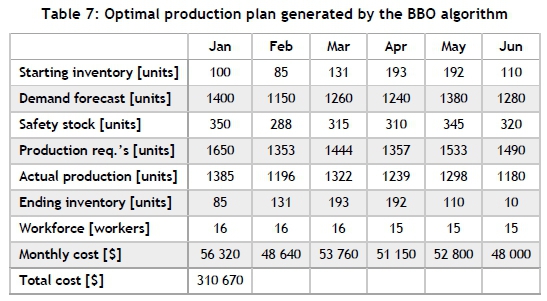
In comparing the total costs of the production plans produced by the BBO and SA algorithms, it was found that the BBO algorithm was able to produce a lower cost plan at $ 310 670.00 than the plan produced by the SA algorithm at $ 312 420.00. The total saving in production cost incurred by the BBO algorithm over the SA algorithm was 0.5 per cent.

 

7 DISCUSSION

Both the BBO and the SA algorithms were able to produce production plans that were superior to the best standard strategy, which was the stable workforce / varying production strategy defined by Chase et al. [3]. When comparing the plans produced by the two optimisation algorithms, the BBO-generated plan had a lower overall cost than the SA-generated plan. The differences in cost savings between the stable workforce / varying production plan, the SA-produced plan, and the BBO- produced plan fell well within the results of Baykasoglu [14] in their comparison of goal programming and heuristic-based methods.

Both the BBO algorithm and the SA algorithm produced plans that turned out to be mixed plans - i.e., a combination of two or more of the standard strategies defined by Chase et al. [3]. This was expected, as the probability of stochastic algorithms such as these producing standard strategies is very low. This also aligned with the prediction of Chase et al. [3] that mixed strategies are usually better than standard strategies.

The best standard strategy plan was based on a constant workforce, whereas the SA generated plan had a non-constant workforce. The algorithm was designed to alternate between constant and nonconstant workforce plans, based on parameters built into the algorithm that varied as the algorithm progressed, and thus converged to the optimal selection between constant and non-constant. The lower cost plan calculated by the SA algorithm showed that there was room for improvement over the standard planning strategies, however small this may have been.

When comparing the workforce levels of the plans produced by the BBO algorithm and by the SA algorithm, it was found that the BBO algorithm also produced a production plan that involved a nonconstant workforce. However, the BBO algorithm was able to produce a plan with less disruption to the workforce, with only a single change from one month to the next over the entire planning period. This was a good result from a human resources perspective, as disruptions to the workforce are not taken lightly by employees. However, it is sometimes the only way for a manufacturer to be economically competitive.

The stable workforce / varying production strategy produced a plan with a fairly high ending inventory, whereas both the BBO and the SA algorithms produced plans with very low ending inventories. One of the main differences between the optimised plans was that the monthly ending inventories of the SA algorithm plan dropped drastically in the third month. This seems to indicate that the cost of holding inventory played a significant role. However, the BBO-generated plan held the monthly ending inventories high until the very last month. The result of the more stable monthly ending inventories of the BBO-produced plan was more stable production requirements, which led to more stable actual production.

From a programming perspective, the BBO algorithm contained more steps than the SA algorithm. However, the BBO algorithm was less computationally intensive than the SA algorithm. The SA algorithm performed 5 000 iterations at each step in the temperature schedule, which required about 1 000 loops per iteration. In contrast, the BBO algorithm only performed 150 iterations, which involved stepping through 100 habitats at each iteration. Furthermore, even though the BBO algorithm was less computationally intensive, it converged to its final output more quickly than the SA algorithm.

 

8 CONCLUSION

In conclusion, the contribution of this research study was twofold. The first was the development of a static simulation mode of an advanced manufacturing system designed to investigate mass customisation manufacturing through single unit order handling. In this study, this model was used as the basis for developing a new production planning optimisation algorithm. The second contribution of this study was the development of this new optimisation algorithm for aggregate production planning. This algorithm was based on the principles of biogeography-based optimisation, which has never been used for this specific application before. This algorithm was able to produce lower cost aggregate production plans than traditional planning methods or an established artificial intelligence algorithm.

 

REFERENCES

[1] Fogliatto, F.S., da Silveira, G.J.C. & Borenstein, D. 2012. The mass customization decade: An updated review of the literature, Int. J. Prod. Econ., vol. 138(1), pp. 14-25.         [ Links ]

[2] Pine, B.J. 1993. Mass customization: The frontier in business competition. Boston, MA: Harvard Business School Press.         [ Links ]

[3] Chase, R.B., Aquilano, N.J. & Jacobs, F.R. 2006. Operations management for competitive advantage, 11th ed. McGraw-Hill, New York, NY.         [ Links ]

[4] MacCarthy, B., Brabazon, P.G. & Bramham, J. 2003. Fundamental modes of operation for mass customization, Int. J. Prod. Econ., vol. 85(3), pp. 289-304.         [ Links ]

[5] Engelbrecht, A.P. 2007. Computational intelligence: An introduction, 2nd ed. Chichester, England: John Wiley & Sons, Inc.         [ Links ]

[6] Xing, B. & Gao, W.-J. 2013. Innovative computational intelligence: A rough guide to 134 clever algorithms. London: Springer.         [ Links ]

[7] Renzi, C., Leali, F., Cavazzuti, M. & Andrisano, A.O. 2014. A review on artificial intelligence applications to the optimal design of dedicated and reconfigurable manufacturing systems, Int. J. Adv. Manuf. Technol., vol. 72(1-4), pp. 403-418.         [ Links ]

[8] Ferreira, J.D. 2013. Bio-inspired self-organisation in evolvable production systems, PhD dissertation, KTH Royal Institute of Technology.         [ Links ]

[9] Stump, B. & Badurdeen, F. 2012. Integrating lean and other strategies for mass customization manufacturing: A case study, J. Intell. Manuf., vol. 23(1), pp. 109-124.         [ Links ]

[10] Simon, D. 2008. Biogeography-based optimization, IEEE Trans. Evol. Comput., vol. 12(6), pp. 702-713.         [ Links ]

[11] Koza, J.R. 1992. Genetic programming: On the programming of computers by means of natural selection. A Bradford Book, The MIT Press, Cambridge, Massachusetts.         [ Links ]

[12] Souier, M., Sari, Z. & Hassam, A. 2013. Real-time rescheduling metaheuristic algorithms applied to FMS with routing flexibility, Int. J. Adv. Manuf. Technol., vol. 64(1-4), pp. 145-164.         [ Links ]

[13] Musharavati, F. & Hamouda, A.M.S. 2011. Simulated annealing with auxiliary knowledge for process planning optimization in reconfigurable manufacturing, Robot. Comput. Integr. Manuf., vol. 28(2), pp. 113-131.         [ Links ]

[14] Baykasoglu, A. 2001. MOAPPS 1.0: Aggregate production planning using the multiple-objective tabu search, Int. J. Prod. Res., vol. 39(16), pp. 3685-3702.         [ Links ]

 

 

Submitted by authors 13 Jun 2017
Accepted for publication 8 Feb 2018
Available online 31 /May 2018

 

 

* Corresponding author Brightg@ukzn.ac.za