GENERAL ARTICLES

 

Risk modelling of heavy mobile equipment to determine optimum replacement ages

 

 

C.F. Kirstein; J.K. Visser^*

Department of Engineering and Technology Management, University of Pretoria, South Africa

 

 

---

ABSTRACT

Maintenance and physical asset managers often have to decide when a major asset needs to be replaced. The main objective of this study was to develop a methodology to determine the optimum replacement age of heavy mobile equipment that is close to the end of its life. The study was conducted on an old electric rope shovel used at a surface coal mining operation. The failure impact and failure probability estimates of components were obtained from subject matter experts through Delphi analyses. A stochastic-and-parametric-estimation modelling solution was developed to perform quantitative risk analyses using their inputs. The solution calculated the expected loss of the rope shovel as a function of machine-age within a 90 per cent confidence interval. The study demonstrated that the optimum replacement age of heavy mobile equipment can be obtained by modelling the expected losses due to the failure of critical end-of-life components, taking into account the uncertainty in data obtained from subject matter experts.

---

OPSOMMING

Fisiese bate- en instandhoudingsbestuurders moet dikwels besluit wanneer om 'n groot bate te vervang. Die hoofdoel van hierdie studie was om 'n metodologie te ontwikkel om die optimale vervangtyd van swaar mobiele toerusting naby die einde van sy leeftyd te bepaal. Die studie was uitgevoer op 'n ou elektriese tougraaf wat by 'n oopgroef steenkool myn aangewend word. Die falings impak en falings waarskynlikhede van komponente is verkry vanaf onderwerpkenners deur middel van Delphi analises. 'n Stogastiese-en-parametriese-beraming modellering oplossing was ontwikkel om kwantitatiewe risiko analises met hul insette te doen. Die oplossing het die verwagte verliese van die tougraaf as 'n funksie van ouderdom bereken binne 'n 90 persent vertrouensinterval. Die studie het getoon dat die optimum vervangingsouderdom van swaar mobiele toerusting bepaal kan word deur die verwagte verliese as gevolg van falings van kritieke komponente naby die einde van hul leeftyd te modelleer, met inagname van die onsekerheid in data verkry vanaf onderwerpkenners.

---

 

 

1 INTRODUCTION

1.1 Background

With expensive capital investments such as electric rope shovels used in mining operations, managers are concerned with the question, "When should we replace the asset?" The engineers in the organisation usually want to replace assets as soon as the risk of severe unplanned equipment failures increases. The financial managers want to replace the equipment as late as possible to keep the cost-of-capital to a minimum. However, the engineers speak in engineering terms (equipment condition) and the financial managers in financial terms (cost of capital), and thus apples are compared with oranges. Both engineers and financial managers need the same consolidated evidence to decide on the best time to replace the equipment.

The optimum replacement age is the machine-age at which the expected losses - i.e., the sum of all costs pertaining to performance, risk, direct costs, and capital expenditure - are the least. The failure impact and failure probability estimates of the electric rope shovel's components were obtained from subject matter experts through Delphi analyses. A stochastic-and-parametric-estimation modelling tool was developed to perform quantitative risk analyses using the inputs from the subject matter experts. The model calculated the expected loss of the rope shovel as a function of machine-age within a 90 per cent confidence interval.

1.2 Research objectives

The objectives of this research study were:

1) To develop a methodology to determine the optimum replacement age of heavy mobile equipment that is close to the end of its life.

2) To apply the methodology to an old electric rope shovel, using mainly subject matter experts (maintenance crew) as the source of data for end-of-life predictions about components.

 

2 LITERATURE AND THEORY

2.1 Life-cycle cost minimisation to determine the optimum replacement age

Du Plessis [1] has shown that managers decide in various ways when equipment should be replaced, but that the majority do so primarily through life-cycle cost minimisation. Life-cycle costing (LCC) is the process of predicting the costs of something throughout its life, starting with acquisition, through operation and maintenance, to final disposal. LCC minimisation keeps the cost of the function or activity throughout the life of the mine as low as possible. Whereas the cost of operations tends to remain more-or-less constant, maintenance costs are volatile, and increase with the age of the asset [2]. Thus maintenance costs are more important than operating costs in LCC analyses.

LCC analyses have been improving since the 1980s, but they are still subjective and inaccurate unless an appropriate method is used [3]. Dhillon [4] and Dhillon and Anude [5] showed that, prior to 1989, all of the LCCs for heavy mobile equipment (HME) were deterministic and treated maintenance costs as a 'fixed' periodic cost or rate. However, a breakthrough in LCC occurred in the 1990s in the form of activity-based costing (ABC) - the process of deriving the LCC from the activities that the asset will perform or the activities that will be performed on the asset. It is generally accepted throughout the literature that activity based life-cycle costing (AB-LCC) is the superior method of conducting LCCs, as it is based on the physics, operations, operating environment, and business processes of the equipment. However, AB-LCC only become achieved prominence in the 21^st century because of the effort and intricacy of maintaining AB-LCC analyses ([1], [3], [6], [7], [8], [9], [10], [11]).

It is almost impossible to determine the optimum replacement age of a particular machine using AB-LCCs, mostly because AB-LCCs are deterministic and a priori in prediction. Richardson et al. [2] (echoed by Emblemsevág [7]) found that, even today, most LCCs are deterministic and unable to accommodate uncertainty, which is a major limitation. Few sources in the literature have found practical applications for stochastic quantitative AB-LCC analyses, and they were not applied with great consistency. Korpi and Ala-Risku [12] state correctly: "Despite existing life cycle costing (LCC) method descriptions and practical suggestions for conducting LCC analyses, no systematic analysis of actual implementations of LCC methods exists ... [M]any of the case study applications covered fewer parts of the whole life cycle, estimated the costs on a lower level of detail, used cost estimates methods based on expert opinion rather than statistical methods, and were content with deterministic estimates of the life cycle costs".

2.2 Predicting the end-of-life to determine the optimum replacement age

Instead of using AB-LCCs, it is better to predict the end-of-life of the equipment to determine its replacement age. But predicting the remaining useful life of something (prognosis) is not the same as predicting the optimum replacement age, or even a priori predictions of the end-of-life [13]. Instead of being static and history-based, prognostics are dynamic and continuously updated with new information [14] to predict the death of an item "to manage business risks that result from equipment failing unexpectedly" [15]. Prognostics are necessary to determine the optimum replacement age, but they present a few challenges.

Firstly, Engel et al. [13] said "Condition-based assessments, the underpinning of the Condition-Based Maintenance philosophy, have usually emphasized the diagnosis of problems rather than the prediction of remaining life. Prognoses are considerably more difficult to formulate since their accuracy is subject to stochastic processes that have not yet happened". Sikorskaetel [15] said: "Most prognostic research work to date has been theoretical, disparate and restricted to a small number of models and failure modes. Unfortunately, there are few published examples of prognostic models being applied in the field, on complex systems, exposed to a normal range of operating and business conditions". Van Horenbeek and Pintelon [14] wrote: "The use of these techniques in maintenance decision-making and optimization in multi-component systems is however a still underexplored area." Engel et al. [13] also said: "Finding where an extrapolated trend meets a condemnation threshold may provide an expectation of remaining life, but it does not provide sufficient information to make a decision". "Many prognostic techniques exist and they are basely classified into three principal classes: data-driven approaches, model-based approaches, experience-based approaches" (Son et al. [16]), but "some models are also not as well proven as others, so the level of risk a business is willing to accept must be understood before implementing a particular modelling approach. In reality, industry sites will also not be able to utilise every prognostic modelling option with equal efficacy" [15].

Secondly, "their ability to perform the modelling and reticulate the outputs to users via existing business systems is dependent on the availability of required data, skilled personnel (in-house or contracted) and computing infrastructure" [15], but prognostic models or techniques rely on highly sophisticated mathematical or theoretical models that are only usable by highly skilled personnel, whereas it should be tractable and accessible to maintenance practitioners [15]. Most prognostic models and techniques are data-dependent - i.e., they are highly sensitive to data quality and quantity; but data may never be in sufficient supply for the models, and the models remain flawed without an opportunity for validation [13], because they can only be verified retrospectively [15].

The challenges can be addressed by ensuring that the uncertainties associated with the calculations are understood, bounded, and accommodated [13], [15]. Current condition information takes precedence over historic failure data or derived information [13], [16]. Since human estimations on complex systems are generally poor, the models should be built on a component level [15]. However, building the model on a component level can increase the uncertainty due to co-linearity [17].

2.3 Quantifying risk to determine the optimum replacement age

Predicting the end-of-life is only useful in determining the optimum replacement age if the risk of failure is quantified (i.e., the probability of failure and the impact of failure), since quantifying the risk enables a cost-benefit view of the equipment nearing its end-of-life. Quantitative risk analysis is preferred over qualitative risk analysis, because qualitative analyses often rely on intuition and 'gut feelings' to determine risk that Kahneman and Tversky [18] and Hubbard and Evans [19] showed to be unreliable. Furthermore, scoring methods or ordinal scales in qualitative analyses almost never have research to validate them [19], and suffer from range compression [20]. Moreover, this study compares performance, cost, and risk; thus it is necessary to quantify risk in terms of money loss. Risk seems to be an elusive concept, and agreement about its definition has not been attained throughout the industry [21]; but common to these definitions is that risk consists of (1) events (scenarios, triggers, or failure modes), (2) consequences (outcomes, severity, or impacts), and (3) probabilities [20], [22]. Of all the risks described by Aven [21], only the expected value (loss) quantifies risk in a monetary value and balances different attributes - namely, consequences and likelihood. The problem with this estimated value (loss), however, is that it does not seem to address uncertainties [21] and it treats the risk decision-maker as risk neutral [20], [22]. Hubbard [20] insists, however, that the uncertainty can be accommodated, and proposes that the components of the expected loss should be kept apart until the risk-averse decision-maker is applied.

2.4 Using subject matter experts to quantify risk

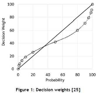
Although quantitative risk models seem to be scientifically correct, they do pose a few challenges. Subject matter experts (SMEs) who are used to quantify the risk are not calibrated by default; thus it has to be assumed that they are systematically overconfiden, and subsequently that the risk is underestimated [20], [23]. Furthermore, they do not have the intuition to estimate failure data for complex systems with inter-related failure modes [15]. But they can and should be calibrated to provide accurate estimates [19], [24]. Kahneman and Tversky [23] maintain that, even with calibrated SMEs, estimation will still be skewed due to cognitive biases, although predictably so with more aversion to their loss than desire to gain [18]. Figure 1 below shows how that plays out with the probability estimations.

 

 

Although certain authors mentioned so far find estimates dubious, many legitimate studies (also mentioned) propose that estimations can be used under certain conditions. The primary condition is that the estimation must be from SMEs, because they understand the underlying mechanisms. Secondly, the SMEs must be calibrated, and their answers adjusted for their bias. Thirdly, the uncertainty of the estimation has to be taken into account, and it must be accurate - which means sacrificing precision.

2.5 Summary of literature review

Life-cycle cost minimisation methods are inadequate when determining optimum replacement ages, despite being the prevalent approach, because they are deterministic, a priori, and unable to accommodate uncertainty.

Prognostic models are not suitable for determining fairly accurate optimum replacement ages, even though they give an indication of the equipment's end-of-life. They have not yet been applied effectively to make management decisions; and they are sensitive to the quality and availability of data.

Risk can be quantified as an expected loss to determine the optimum replacement age, and prognostic models can be used to assist in quantifying risk. The challenge lies in managing uncertainties and risk neutrality.

Subject matter experts can be used to quantify the risk - i.e., perform end-of-life predictions and quantify the impacts of failures. The challenge is to assure the accuracy of their estimates.

 

3 RESEARCH METHODOLOGY

3.1 Conceptual framework for methodology

Equipment performance, direct costs, and risk could be compared by quantifying each as a cost or a loss. The expected loss model can be applied to any equipment nearing its useful end-of-life or any major maintenance intervention to determine an optimal age at which the event should occur.

This study used an ageing electric rope shovel at 109 000h of age at an open cast coal mine as a case study to demonstrate the methodology of selecting the optimum replacement age. The conceptual framework of the methodology is explained through the following steps:

1. Develop risk analysis method and model

• Select best risk analysis method

• Create stochastic & parametric estimation risk model

2. Determine equipment risk

• Identify end-of-life (EOL) components

• Estimate impacts of EOL component failures

• Estimate probabilities of EOL component failures

• Determine equipment risk

3. Determine equipment expected loss

• Determine the expected loss as a function of age, using Monte Carlo simulation

• Determine whether the uncertainty is small enough to be useful to decision-makers and managers

The overall conceptual framework is illustrated in Figure 2 below.

 

 

3.2 Acquiring data

When failure data is available, there are several methods to analyse the data and apply it to estimating failure probability [15]. Most reliability engineering research seems to be built on the analysis of measured data. However, even though this study addresses the 'what-if-you-have measured data' question (see, for example, section 4.2.1 ), it attempts mostly to answer the 'what-if-you-don't-have (measured) data' question.

As mentioned in section 2.4, any estimate should be accurate before it is precise - i.e., the true value must be within the range of uncertainty. Only once this is assured can the precision (range of uncertainty) be improved through further measurement [24]. All estimate methods - data, model, and experience [16] - can be accurate, but they are not equally precise. Measured data is expected to be the most precise; then suitable (theoretical) models of failure mechanisms; then the experience of SMEs. This approach is illustrated in Figure 3, and each type is discussed in some detail in the following paragraphs.

 

 

3.2.1 Measured data

Measured failure data is difficult to obtain and, even when obtained, it does not provide a probability of failure. The data must still be transformed from diagnosis to prognosis [13], [14]. The challenge with prognosis is that it requires regular (if not continuous) updates to detect a trend that it can extrapolate to a certain threshold. If the threshold is not known, or if there are only one or two points of reference in time, the measured data becomes unusable. In this study, measured data was available; it is evaluated in paragraph 4.2.1.

If the measured data were not available, or were insufficient for a prognostic model, the next best option would be to simulate the measured data. This introduces the next issue: modelling failure mechanisms.

3.2.2 Modelling component failure mechanisms

Finite element analysis (FEA) has developed substantially over the past decade to model failure mechanisms. FEA can model cracks in complex materials such as laminates with consistent accuracy [25]; and Rabczuk et al. [26] have shown that it has become computationally cheaper, by applying smoothing techniques to overcome very distorted meshes, thus not requiring constant remeshing. But there are two limitations.

Firstly, the accuracy of the prediction is highly sensitive to the loading input [25]. Any model that is built to simulate the rate of crack propagation would need an accurate load-over-time input, which means that data has to be gathered, over the life of the HME, about the loads the components were exposed to; otherwise the loads would have to be simulated as well. Gu et al. [27] modelled an A-frame for a mining dump truck where the route was analysed and used as inputs to the FEA. For a rope shovel, there are two factors that especially affect the loading on the structural members: floor condition and operator behaviour. Poor floor conditions cause excessive rocking, thereby aggravating the intensity and frequency of loads on the structural members. Furthermore, poor operator behaviour causes excessive break-out force to be applied: the booms loaded laterally to clean the floor impact with the truck; excessive tramming; and so forth. Operators also change from shift to shift and between shovels.

Secondly, although cheaper than previously, it is still expensive when numerous components, each with numerous failure modes, need to be simulated. For example, the rope shovels have more than 600 components (sub-assemblies and lower) with various inter-dependencies. Even simulating 31 EOL components per shovel would require expertise, time, and money that managers would be loath to spend. Time is especially constrained. In this study, there was no simulated data to use. If the modelling data were not available or were insufficient for a prognostic model, the final option would be to obtain the opinions from subject matter experts (SMEs).

3.2.3 Experience of subject matter experts (SMEs)

Inputs from SMEs can be obtained through Delphi analyses [28]. The approach followed in paragraph 4.2.3 is as follows:

1. Identify the EOL components

2. Calibrate the SMEs

3. Using Delphi analyses, obtain estimates of

   • the impact of a failure for each component

   • the probability of a failure

4. Use inference for wear-out phases of components

 

4 RESULTS

4.1 End-of-life components

The critical end-of-life (EOL) components have a high impact on the machine's reliability, meaning that, if these components become unreliable, the performance of the heavy mobile equipment (HME) is severely reduced. Subject matter experts were involved in the identification of 31 EOL components of the electric rope shovel. Maintenance personnel responsible for the rope shovels were regarded as the experts in this case. An example of the data captured for some of the critical EOL components is shown in Table 1.

 

 

4.2 Data collection

4.2.1 Measured data

The condition of the shovel was evaluated, and cracks were identified in its structural members. The most affected areas were revolving frames, under-carriages, booms, and crawler frames. The total crack length was about four times more than it was at 30 000h, according to the maintenance staff. However, there is no known threshold for the crack lengths beyond which it can be said that the shovel cannot be operated further. Oil and thermographic readings since 2007 were taken on various components, but since the oil and electric circuits were replaced, this was again not useful in determining the EOL of the shovel.

4.2.2 Experience of subject matter experts

The SMEs for the rope shovels are the maintenance personnel: the head of maintenance, the foremen, and the master artisans. Six persons were selected for this study. Each of these SMEs had more than eight years' experience working on these shovels, and all but one were involved in the previous rebuild of the rope shovel at 109 000 hours.

For the consequences or impacts of failures, the SMEs were simply asked to tell a 'story' of what would happen if the component failed. They were asked to consider:

• Direct maintenance costs - the cost of repairing or replacing the component (salaries or rates not to be included).

• Amount of downtime that will be incurred - do you have spare components, or do you have to place orders and wait? How long will you wait, and how long will it take once you have the item?

• Sequential and collateral damages - what is the chance of damaging other components of the rope shovel?

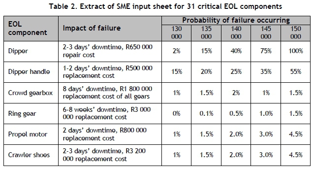
Each SME was given an input sheet to populate before the work session was held. An extract of the input sheet is shown in Table 2.

For each of the machine ages indicated in Table 2, the SMEs were asked to estimate the chance of failure of the component. Their estimates are cumulative conditional probability of failures, since they consider that a component has survived up to a certain year, and what the likelihood of failure will be in that year. Once the input sheets were received, a workshop was held with the SMEs, during which the following actions took place:

• The personnel had not been calibrated for guessing prior to the study; therefore over-confidence was explained, and some exercises were done to calibrate them.

• The estimates of the SMEs were shared with each other (anonymously), and the validity of the answers was checked.

• The SMEs were then given the opportunity to revise their estimates.

For this study, only the EOL components were modelled. Any failure on the structural members would have caused the HME to be replaced instead of repaired. Also, the possible collateral damage had been taken into consideration with impact trees. The stochastic dependencies were treated as competing risks (or multiple decrements), and so could be treated as a series system of components [30], [31]. There was no foreseen correlation or subsequent co-linearity between the components of the shovel.

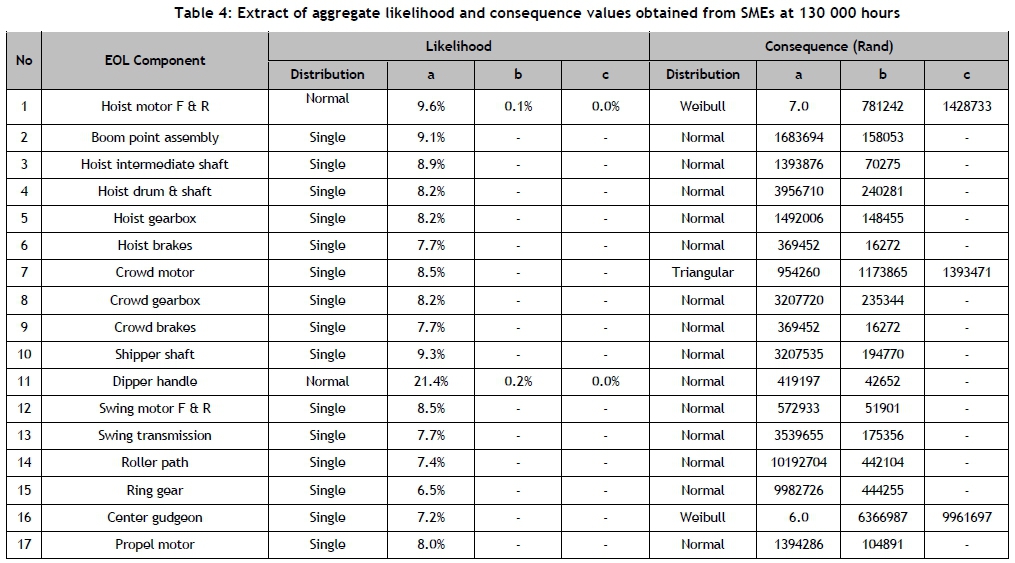
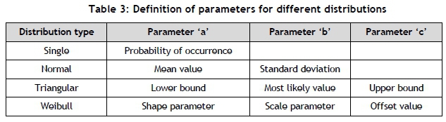
All the inputs obtained from the SMEs were aggregated into single distributions for the failure probability and failure impact (shown in Table 4). The inputs were simulated in the model through Monte Carlo analyses, with each failure probability and impact simulated 10 000 times per component. Table 3 gives the meaning of a, b, and c in Table 4 for the different distributions used.

4.3 Data processing

4.3.1 Introduction

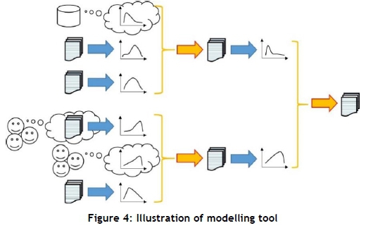
The study developed a modelling tool that essentially performs two functions: parametric estimation and stochastic modelling. The parametric estimation function aggregates data sets into parametric functions; and the stochastic modelling creates new data sets from a combination of parametric functions. Figure 4 below illustrates how the parametric estimation (blue arrows) and stochastic modelling (orange arrows) work together to model risk.

 

 

The critical EOL components have a high impact on the machine's reliability, meaning that if these components become unreliable, the HME's performance is severely reduced. In this case, 31 EOL components were identified and evaluated.

The risk for each component was calculated from equation 1.

where:

P_fail tail is the probability of the component failing

C_i is the i^th impact of the component failing

P_i is the probability of the i^th impact occurring

k is the total number of impacts in the impact tree

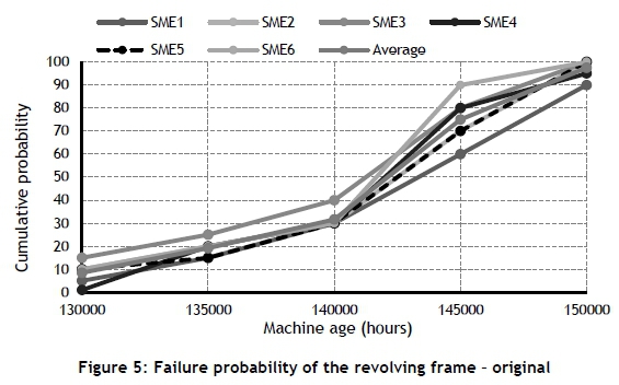
Often risk impacts cause chain reactions; so the modelling tool allowed an impact tree to be built that included the interdependencies of the impacts. The inputs to build impact trees were obtained from engineers in the company. The probabilities of failures were obtained from the maintenance crew of the electric rope shovel. An extract of their inputs for the revolving frame assembly, with adjustment for their bias, is shown in Figures 5 and 6.

 

 

 

 

The expected loss is calculated by adding the change in the cost of capital to the risk, as indicated in equation 2.

where ΔCoC is the change in the cost of capital.

It was assumed that the capital would have been spent at 150 000 hours to replace the electric rope shovel. Earlier replacement is deemed a 'cost' with a discount rate of 10% pa. All of the uncertain inputs - the probability of failures, and the consequences of such failures - for all 31 EOL components were combined in a Monte Carlo cost risk simulation. The simulations were repeated at 130 000 h, 135 000 h, 140 000 h, 145 000 h, and 150 000 h of machine age. This simulation can often be performed in an MS Excel spreadsheet; but for this research project, a stand=alone software program was developed. The output of a cost risk simulation is typically a cumulative distribution function (CDF) for the total expected loss at a certain time or machine age. The expected loss - i.e., the sum of the risk of failure and Δ cost of capital - can be determined from the simulation output at various probability or confidence levels - e.g., 5%; 25%; 50%; 75%; and 95%. The expected loss for a 50% confidence level is shown in Figure 7 as an example.

 

 

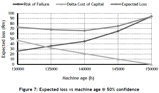
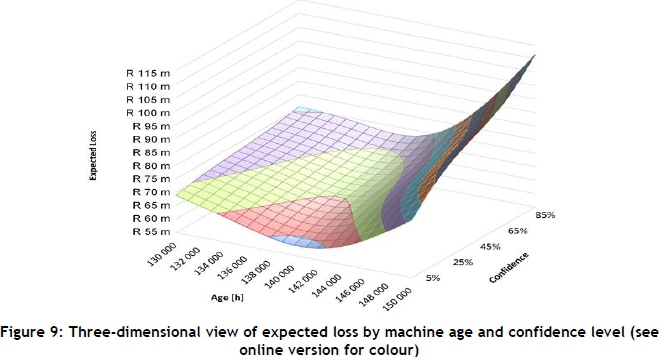
The minimum expected loss at 50% confidence level is at about 140 000 hours machine age. The expected loss was determined for various machine ages and confidence levels, as shown in Figures 8 and 9 below.

 

 

The 90% confidence age-window is surprisingly small, and is not very sensitive to fluctuations in the risk estimation and discount rates. The managers found that the four-month window was an adequate basis for their decisions.

The SMEs found this process very intuitive. They are more used to guessing in ranges - e.g., "about 6 to 8 weeks" - than providing exact values. In fact, when they are forced to provide exact figures, they are inclined to provide the worst-case scenarios in order to be certain.

 

5 CONCLUSIONS

The results show that it is possible to obtain a 90% confidence age-window in which the true minimum expected loss resides. The expected loss took into account direct costs such as the cost of capital, component repair/replacement costs, and contractor costs. The study quantified the performance as a loss of production and the subsequent loss in profits. The sum of direct costs and performance loss is the quantified risk.

The study found that accuracy and precision are not the same thing. One can be accurate but not precise; or precise but not accurate. The preference was to obtain accuracy even though the uncertainty could be unbearably large. This study applied proven quantitative risk methodologies to a case study. The errors and limitations of the method were identified and discussed throughout the study, where they were managed appropriately.

The study obtained most of the inputs to the risk model from subject matter experts (SMEs) through Delphi analyses. The SMEs were treated as biased agents, and appropriate corrections were made to their estimates to ensure the consistency and accuracy of the information.

The precision of the results was acceptable for practical application. The 90% confidence age-window in which the true minimum expected loss resides was about four months. The management team would have been happy with a window of 12 months, or even 18 months.

The method to determine the optimum replacement age of the rope shovel assembly can be applied to other equipment. In fact, this approach and methodology can be applied to any replaceable system with deteriorating end-of-life components.

 

REFERENCES

[1] Du Plessis, C. 2007. Replacement of earthmoving equipment at surface mining operations in South Africa. Dissertation for MBA, Gordon Institute of Business Science, University of Pretoria.         [ Links ]

[2] Richardson, S., Kefford, A. and Hodkiewicz, M. 2013. Optimised asset replacement strategy in the presence of lead time uncertainty, International Journal of Production Economics, 141(2), pp 659-667.         [ Links ]

[3] Kayrbekova, D., Markeset, T. and Ghodrati, B. 2011. Activity based life cycle cost analysis as alternative to conventional LCC in engineering design, International Journal of System Assurance Engineering and Management, 2(3), pp 218-225.         [ Links ]

[4] Dhillon, B. 1989. Life cycle costing - Techniques, models and applications. Gordon and Breach Science Publishers, New York.         [ Links ]

[5] Dhillon, B. and Anude, O. 1992. Mining equipment reliability - A review, Microelectronic Reliability, 32(8), pp 1137-1156.         [ Links ]

[6] Charles, S. and Hansen, D. 2008. An evaluation of activity-based costing and functional-based costing: A game-theoretic approach, International Journal of Production Economics, 113(1), pp 282-296.         [ Links ]

[7] Emblemsevåg, J. 2003. Life-cycle costing: Using activity-based costing and Monte Carlo methods to manage future costs and risks. John Wiley & Sons, Hoboken, New Jersey.         [ Links ]

[8] Fichman, R. and Kemerer, C. 2002. Activity based costing for component-based software development, Information Technology and Management 3(1), pp 137-160.         [ Links ]

[9] Pike, R., Tayles, M. and Mansor, N. 2011. Activity-based costing user satisfaction and type of system: A research note, The British Accounting Review 43(1), pp 65-72.         [ Links ]

[10] Kallunki, J.P. and Silvola, H. 2008. The effect of organizational life cycle stage on the use of activity based costing, Management Accounting Research 19(1), pp 62-79.         [ Links ]

[11] Langmaak, S., Wiseall, S., Bru, C., Adkins, R., Scanlan, J. and Sobester, A. 2011. An activity-based- parametric hybrid cost model to estimate the unit cost of a novel gas turbine component, International Journal of Production Economics, 142(1), pp 74-88.         [ Links ]

[12] Korpi, E. and Ala-Risku, T. 2008. Life cycle costing: A review of published case studies, Managerial Auditing Journal, 23(3), pp 240-261.         [ Links ]

[13] Engel, S., Gilmartin, B., Bongort, K. and Hess, A. 2000. Prognostics: The real issues involved with predicting life remaining, Aerospace Conference Proceedings, IEEE, Volume 6, 18-25 March 2000, pp 457-469.         [ Links ]

[14] Van Horenbeek, A. and Pintelon, l. 2013. A dynamic predictive maintenance policy for complex multi-component systems, Reliability Engineering and System Safety, 120, pp 39-50.         [ Links ]

[15] Sikorskaetal, J. 2011. Prognostic modelling options for remaining useful life estimation by industry, Mechanical Systems and Signal Processing, 25(5), pp 1803-1836.         [ Links ]

[16] Son, K., Fouladirad, M., Barros, A., Levrat, E. and Lung, B. 2013. Remaining useful life estimation based on stochastic deterioration models: A comparative study, Reliability Engineering and System Safety, 112, pp 165-175.         [ Links ]

[17] Hager, J., Yadavalli, V.S.S. and Webber-Youngman, R. 2015. Stochastic simulation for budget prediction for large surface mines in the South African mining industry, Journal South African Institution of Mining & Metallurgy, 115(6), pp. 531-539.         [ Links ]

[18] Kahneman, D. and Tversky, A. 1979. Prospect theory: An analysis of decision under risk, Econometrica, 47(2), pp. 263-292.         [ Links ]

[19] Hubbard, D. and Evans, D. 2010. Problems with scoring methods and ordinance scales in risk assessment, IBM Journal of Research & Development, 54(3), 2^nd paper.         [ Links ]

[20] Hubbard, D. 2009. The failure of risk management: Why it's broken and how to fix it. John Wiley & Sons Inc., Hoboken, New Jersey.         [ Links ]

[21] Aven, T. 2012. The risk concept - Historical and recent development trends, Reliability Engineering and System Safety, 99, pp 33-44.         [ Links ]

[22] Aven, T. 2010. On how to define, understand and describe risk, Reliability Engineering and System Safety, 95, pp 623-631.         [ Links ]

[23] Kahneman, D. and Tversky, A. 1974. Judgement under uncertainty: Heuristics and biases, Science, New Series, 185(4157), pp. 1124-1131.         [ Links ]

[24] Hubbard, D. 2010. How to measure anything: Finding the value of intangibles in business, John Wiley & Sons Inc., Hoboken, New Jersey.         [ Links ]

[25] Duran, J. and Hernandez, C. 2014. Evaluation of three current methods for including the mean stress effect in fatigue crack growth rate prediction, Fatigue & Fracture of Engineering Materials & Structures 38(4), pp 410-419.         [ Links ]

[26] Rabczuk, T., Bordas S. and Zi, G. 2010. On three-dimensional modelling of crack growth using partition of unity methods, Computers and Structures, 88, Issues 23-24, December, pp 1391-1411.         [ Links ]

[27] Gu, Z., Mi, C., Wang, Y. and Jiang, J. 2012. A-type frame fatigue life estimation of a mining dump truck based on modal stress recovery method, Engineering Failure Analysis, 26, pp 89-99.         [ Links ]

[28] Rowe, G. and Wright, G. 1999. The Delphi technique as a forecasting tool: issues and analysis, International Journal of Forecasting, 15, pp 353-375.         [ Links ]

[29] Kahneman, D. 2011. Thinking, fast and slow, Farrar, Straus and Giroux, New York.         [ Links ]

[30] Leemis, L.M. 2009. Reliability: Probabilistic models and statistical methods. Lawrence Leemis, 2^nd edition, Williamsburg.         [ Links ]

[31] Gooley, T., Leisenring, W., Crowley, J. and Storer, B. 1999. Estimation of failure probabilities in the presence of competing risks: New representation of old estimators, Statistics in Medicine, 18(6), pp. 695-706.         [ Links ]

 

 

Submitted by authors 6 Jul 2016
Accepted for publication 20 Sep 2017
Available online 13 Dec 2017

 

 

* Corresponding author krige.visser@up.ac.za