GENERAL ARTICLES

 

An approach to improving marketing campaign effectiveness and customer experience using geospatial analytics

 

 

M.P. Brink^#; A. van Rensburg^*

Department of Industrial Engineering, Stellenbosch University, South Africa

 

 

---

ABSTRACT

This article discusses a case study in which a South African furniture and household goods retailer wishes to improve its marketing campaigns by employing location-based marketing insights, and also to prioritise customer satisfaction. This paper presents two methods used in an exploratory exercise with the aim of improving the retailer's business in these ways. The methods of customer profiling and identifying geographical customer clusters summarise how the retailer's strategic marketing strategies and customer experience can be improved. The methods presented in this article rely on the use of spatial data to solve the business problems.

---

OPSOMMING

Hierdie artikel bespreek 'n gevallestudie waarin 'n Suid-Afrikaanse meubel-en-huishoudelike goedere handelaar beoog om hul bemarkingsveldtogte te verbeter deur plek-gebaseerde bemarkingsinsigte, en verder, om kliënt-tevredenheid te prioriteseer. Hierdie artikel stel twee metodes voor, wat toegepas word in 'n verkennende oefening met die doel om die kleinhandelaar se besigheid te verbeter. Die skepping van kliënteprofiele en die identifikasie van geografiese-gebaseerde kliëntebondels wys hoe die kleinhandelaar se bemarkingstrategië en kliënt-tevredenheid verbeter kan word. Die metodes in hierdie artikel maak gebruik van ruimtelike data om die kleinhandelaar se besigheidsprobleme op te los.

---

 

 

1 INTRODUCTION

The high level of competition in, and the rapid pace of, the South African business environment make retaining customers and gaining market share a challenging task. Applying the knowledge gained from customer insights can be the differentiating factor in gaining market share over competitors. In an environment where data are readily available, and in large quantities, the use of business intelligence defined by customer insights becomes an important asset. According to Daniel [2], a short-coming in business intelligence worldwide is that there is so much data, but too little insight. Daniel [2] supports this statement by quoting Bill Hostmann, a Gartner research analyst: "Everything we use and buy is becoming a source of information and companies must be able to decipher how to harness that". One reason to harness business intelligence is to understand how this intelligence influences customer satisfaction. In their White Paper, Frost and Sullivan [4] state that, in regular interactions with customers via multiple communication channels, there is ample opportunity to reduce costs significantly and to enhance customer satisfaction. Frost and Sullivan [4] also state that a top industry trend is the prioritisation of customer satisfaction, retention, and loyalty.

This article discusses a case study in which a South African furniture and household goods retailer wishes to improve its marketing campaigns by employing location-based marketing insights, and to prioritise customer satisfaction. The retailer's current business model poses two problems. The first arises from the retailer's lack of understanding of who its customer is. Given the limited amount and quality of customer data that are acquired at the point of sale, the retailer would like to gain insight into its customers. This insight will create a better customer experience by enhancing customer-product associations. The second problem is the inability of the retailer's marketing team to develop specific location-based marketing campaigns. This problem arises from data that is limited, resulting in a limited understanding of where and how the customers are geospatially located. The objective of this study is to address these problems, and to provide a solution based on data mining and modelling techniques.

 

2 DATA HANDLING

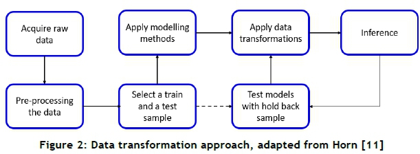
This chapter discusses the extraction, transformation, and loading (ETL) process of data, and presents a flow diagram of how the data used in this study are segmented and selected for experimentation. Theodorou et al. [21] state that ETL processes play an important role in supporting modern business operations that are centred on artefacts (data) that exhibit high variability and diverse lifecycles. In this research, spatial data are transformed at multiple stages of their life cycle in order to create clusters, relationships, and a host of measures that define these relationships. Figure 1 is a conceptual view of the ETL process.

 

 

ETL is a key process for data management and control, and facilitates the process of data storage [23]. This article, however, evaluates a static snapshot of data that have been extracted from a system. In a recent presentation at an R-Users Meetup, Horn [6] and Manjunath et al. [11] presented an approach to data transformation that precedes the load phase of the ETL process - presenting data in a logical format. This approach is shown below.

 

Figure 2

 

The initial step, acquire raw data, proceeds from the extract phase in the ETL sequence. Several steps are then iteratively applied to the data to achieve the required transformations. One of these steps, select a train and a test sample, splits the data into two samples to produce two semantic layers of data that are produced from the transform phase. The reason for this is two-fold. The test sample is the validation sample, and is used to test how a new set of data performs under the same model¹ parameters. The second reason is to ensure that the model used is robust and reliable. In their study on sampling techniques for data testing, Manjunath et al. [11] present a case for cluster sampling, in which train and test samples are selected by virtue of subgroups, such as geographic locations, over a consistent period of time. Data transformations are applied to the sample data in order to fit the models more accurately and to make sense of the data by eliminating 'noise' [10]. The next two sections of this chapter will define which data are extracted and used in this research, and how the train and test samples are identified to achieve the objectives stated in this article.

2.1 Data sources

2.1.1 Internal data

In the Introduction, several problems faced by the retailer were described, and a brief overview of the operational processes that drive the retailer's business was presented. A large international logistics company, the custodian of the retailer's delivery information, provided a sample of the retailer's customer data that was used to conduct this study. The customer data consist of proof-of-delivery (POD) information for deliveries of goods purchased by a host of customers throughout South Africa. Table 1 shows an example of the POD information provided.

 

 

These data are considered to be internal data, as they are acquired from the retailer's Enterprise Resource Planning (ERP) system, and contain sensitive information about the retailer's business. Due to the sensitivity of the complete internal data set (customer identity, transaction information, contact numbers, etc.), only the fields shown in Table 1 were provided for the research conducted in this article. Given that the information in Table 1 is somewhat limited, external data have been used to supplement this data to replace sensitive customer information with an alternative.

2.1.2 External data

In this study, 'external data' refers to any data that are not directly related to the retailer's customers. The purpose of using external data is ultimately to understand the internal data better, by using the properties of the external data that can be matched to the customer information. Two external data sources are used in this study: population data and geospatial data.

Population data: Population data are acquired from Statistics South Africa [19], and consist of data that describe living conditions in South Africa. These data are accumulated every five years, using a survey that aims to identify and profile poverty in South Africa. They give policy-makers information on who is poor, where the poor are located, and what drives poverty in the country [19].

Geospatial data: York University Libraries [24] define 'geospatial data' as data that identify the geographic location of features and boundaries on Earth. These features include natural features, oceans, rivers, etc. Spatial data are generally stored as coordinates (latitude and longitude points) and topology. One such example of geospatial data is shapefiles. Shapefiles for numerous countries have been developed by the Environmental Systems Research Institute, Inc. (ESRI) [3].

2.2 Data samples

Following the data selection approach proposed by Manjunath et al. [11], an appropriate train and test sample is selected. However, before selecting samples from the data, the parameters that constrain the study presented in this article need to be defined. The parameters of the internal data set used in this study are given below.

The constraints of the test and train samples are defined in Table 3. The constraints in Table 3 show that only customer deliveries in Gauteng, South Africa are considered in this research. A date range of six months has been used for both samples (50:50). The reason for the geographical constraint is to simplify the results of this study by evaluating customer deliveries in one province rather than in several. A 50:50 split has been selected, based on the logic that an uneven split of the data might result in the test sample not having sufficient customer data to match the population data attributes.² This is an initial assumption that is verified in the results.

 

 

 

 

3 METHODOLOGY

This article introduces a method both to profile the customers and to identify and interpret customer clusters. In Section 2, the necessity of a software tool for handling spatial data is mentioned. All computations referred to in this article are performed using R software (version 3.2.5) [16], a statistical programming language that supports numerous libraries containing embedded functions that support the computation of complex algorithms.

3.1 Customer profiling

This section discusses how profiles are created for customers in Gauteng. The profiles are based on population census data that include a host of descriptive fields about the population of Gauteng. The objective of profile creation is to produce a view of what the 'average' customer looks like, for certain administrative regions of Gauteng. Section 2 mentioned the use of shapefiles (acquired from the Municipal Demarcation Board [12]) that can be used to identify the administrative boundaries of a country or region. The shapefile for South Africa contains boundaries at various degrees of granularity, ranging from provinces to electoral wards. Given that the scope of the customer data used in this research is limited to Gauteng, customers will be profiled at a municipal district level within the province of Gauteng. Therefore, for each of the six municipal districts of Gauteng, a profile will be created that best depicts the attributes of that district's population. In order to do this, the most granular administrative boundary containing a customer location should be used for accurate depictions. The electoral ward in which each customer resides will therefore be used to identify individual customer attributes. The population data of these wards are projected on to the customers so that the following statement can be made about each customer: customers are assumed to exhibit the attributes of the population of the electoral ward in which they reside. Following this assumption, a second statement can be made about a group of customers residing in a larger area; customers are assumed to exhibit the average attributes of all the customers³ in that region. The steps applied to producing customer profiles (based on the two listed assumptions) are described below:

1. Determine both the district and the most granular administrative boundary (i.e., electoral ward) in which each of the customers in the sample area resides.

2. Identify the characteristics of the average customer for each electoral ward.

3. Determine the characteristics of the average customer for each municipal district of Gauteng.

3.1.1 Determining administrative boundaries

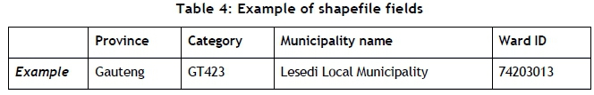
The requirement for the first step in the methodology for customer profiling is to determine in which administrative area each customer address exists, both at district and electoral ward level. To do this, the shapefile containing all administrative areas for South Africa is used. The library rgdal in R is used to import the data in the shapefile and read its contents, which consist primarily of lists of boundary coordinates at a provincial, municipal district, and electoral ward level. This shape contains the fields shown in Table 4.

 

 

A function is required that assigns a ward identity to each customer by computing whether or not each customer address is contained within the boundary point of each ward. This is computed using the point.in.polygon function from the sp library [13] in R. The function verifies, for one or more coordinate points, whether they are contained within a given polygon or boundary [16].

The output of this function is a vector containing a ward identity (ID) corresponding to each customer address in the sample. Wards, which are associated with municipalities (see Table 4), are now linked to individual customer addresses. A frequency count is performed on the number of customers within each ward, and this number is associated with each unique ward ID.

3.1.2 Identifying customer characteristics

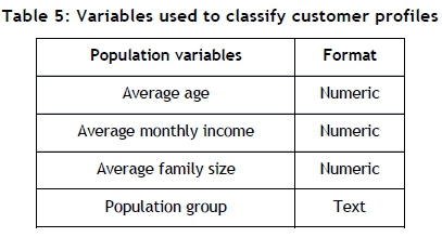
Statistics South Africa [19] provides several fields of information about the population of South Africa. For the objectives of this research, the following four fields are used to create customer profiles of the retailer's customer base in Gauteng.

These four indicators have been chosen in this study because they provide a good representation of the type of product that the customer will be interested in, based on age, population group, and family size, and an affordability indicator of products in different parts of Gauteng. Note that the mean values for each field have been deduced from the population numbers provided by Statistics South Africa [19].

3.1.3 Determining customer characteristics (district level)

This section shows how population characteristics are projected on to customers in proportionate measures. For example, given a sample of 200 customers living in various wards within a municipal district, if 50 of these customers reside in Ward A, then 25 per cent (⁵⁰/200) of Ward A's population data are attributed to the profile of the average customer for that municipal district. This proportion of customers per ward versus the total number of customers per district is multiplied by the number of customers in each ward. The calculation is shown below:

where:

X_jk= average proportionate population of field k for district j

c_i; = customers in ward i

d_j = customers in district j

w_ik= population values of field k for ward i

By applying equation (1), the values of all four population data fields are attributed to the retailer's average customer who lives in each respective municipal district.

3.2 Determining and interpreting clusters

This next part of the methodology addresses the problem of supporting a location-based marketing strategy for the retailer. Given the fact that spatial data about customers are used in this research, the grid-based cluster method proposed by Han and Kamber [5] is most appropriate for identifying the clusters. The grid-based clustering method is recommended when using spatial data on a point coordinate system [22]. This method relies on the application of a m ₓ n grid that is applied to a sample area or window. The grid therefore overlays the sample area and records the number of objects contained within each element or bin of the grid. Bins with higher object counts are more densely-populated (in terms of object per unit area) than bins with lower object counts. This statement can be made because the bins are all exactly the same size.

3.2.1 Grid dimensioning

The information about customer clusters that is produced by this method needs to be interpretable; thus the bins cannot be too large or too small in size and number. Logically, if a large area - for example, 20 000 km² consisting of more than 20 000 objects - were segmented by a very small number of bins (e.g., 10 bins), then the objects contained in each of those ten bins would not add significant value to the information about the density of the area. Conversely, having a large number of bins (e.g., 10 000 bins) would result in data that were too granular. Equally, a large number of bins each containing few or no objects would distort the identification of densely-populated areas by flooding the information with a micro-segmented area. In the context of this study, the aim is to segment the sample area of Gauteng to produce location-based marketing information that is of practical use to the retailer. Thus an optimal bin size needs to be selected to produce areas of the retailers' customers that can be penetrated by marketing campaigns. Scott's [18] rule determines an optimal bin size, using a multi-dimensional histogram, for the sample area of Gauteng.

Scott's [18] formula produces a matrix that contains 55 bins in the latitudinal (vertical) direction and 47 bins in the longitudinal (horizontal) direction. This equates to 2 585 bins in total, each having a surface area of 9.84 km². The grid is applied to the sample area by specifying the above-mentioned dimensions. The grid is created (in R) in the form of a spatial object that contains the following elements:

• The coordinate points of each bin.

• The number of customers from the sample contained in each bin.

• The probability density function for the customers contained in each bin.

A quantitative analysis of high-density areas at a granular level will enable the retailer to pinpoint key areas of interest. While customer density per unit area is a useful measure of density, determining the measure of how clustered customers are requires additional computation, above simply counting the number of customers per bin. The variance of the distances from all the customers in a bin to that bin's mean customer presents quantitative measures of low and high variance bins. The steps followed in determining the variance of each bin are summarised below.

1. Calculate the mean customer coordinates for each bin.

2. Calculate the distance from each customer to the mean customer coordinate of each bin.

3. Calculate the variance of each bin by using the distance measures.

While the steps listed above may seem computationally taxing, R provides several libraries that accommodate these calculations. The mean coordinates of each bin are calculated by applying the mean function in R that exists in the base libraries. Given that there are 2 585 bins and more than 25 000 customers in the test sample area, the sapply and split functions from the R base library enable the application of the mean function over groups, which in the case of the customer data base are bins. The mean latitude and longitude points for each bin are used in a function that calculates the distance from each customer coordinate to the mean coordinates, and calculates the variance using the base var function in R.

The output of the function described above is a variance measure (of the distances from each customer to the mean location) of each bin. This variance measured is organised from the least to the most variance to identify the most- to the least-clustered bins.

Cluster inference

This section evaluates several population variables to determine why customers are significantly clustered in some bins, but not so much in others. The variable(s) that account for clustering are called the propounding variables. These variables are identified using a multivariate analysis, in which the principal components of the sample data set are extracted and evaluated for their contribution to low- or high-variance bins. Once the propounding variables are identified in the multivariate model, the test data sample is plugged into the same model to test how the model performs, given a new data set. In order to build a model that can evaluate the effect of population data variables on the variance of bins (which contain customer locations), the population data need to be transformed so that each bin contains a unique (mutually exclusive) set of population data.

3.2.2 Data transformation

Census data are stored in groups of uniquely-shaped polygons determined by administrative boundaries (wards, municipal districts, etc.). Bins, however, are defined by different parameters - those that are in the grid-cluster method. The population data need to be projected on to the bins to assess the population characteristics of the area defined by each bin. The population data therefore need to be transformed from their current grouping of variables (by administrative areas) to the bins' parameters. This can be achieved by assigning population data to bins in the proportion in which customers can be assigned to bins. The administrative boundaries of 'electoral' wards are used for data projection, as these are the most granular form of boundary available, and therefore the most useful in projecting accurate proportions. Figure 3 illustrates this.

 

 

Figure 3 shows an example of multiple customers found in one bin. These customers exist in two wards simultaneously, each with their own population information. The boundaries of the wards and bins intersect at several places, and portions of both wards are found within the bin. The aim is to project the population data from the wards on to the bins, according to some logical approach. The customers can be used to select a subset of both wards' population data proportionately for projection on to the bin. In this example, one-quarter of all the customers in Bin 1 are in Ward 1, and the remaining three-quarters in Ward 2. Therefore, 25 per cent of Ward 1 's population data and 75 per cent of Ward 2's population data will be projected on to Bin 1. This method of proportioning the data ensures that each bin contains the population data from one or more wards, contributed by mutually-exclusive customers.

The output of this data transformation procedure produces a table containing the aggregated proportion of population data from all wards, for each unique bin. Each bin now has several fields of population data assigned to it, as well as a variance measure.

The next section involves data exploration to test whether or not any of the population data are responsible for the measure of variance in each bin.

3.2.3 Multivariate analysis

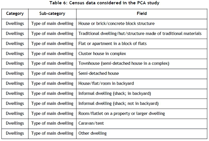
In this section a principal component analysis (PCA) is performed to identify one or more propounding variables in the data that account for customer clusters. The census data that are considered in this study contain more than 100 fields of descriptive living conditions of the population of South Africa. The PCA is performed on a subset of these variables, based on logical selection; this is discussed later in this section. The multivariate analysis (performed using the PCA) tests the validity of the research question that is asked in this study: Are the factors that cause customer clusters those pertaining to the infrastructure of customers' residences - i.e. the classification of the residence? This research question is based on the logic that customers who reside in large, free-standing properties are more likely to be dispersed than customers who reside in more confined residences such as clusters, complexes, or apartments.

To answer that research question, all population variables pertaining to the type of dwelling of people will be considered in the PCA. These variables are shown in Table 6.

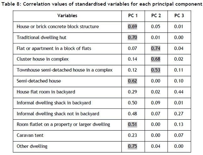
There are two libraries in R that cater for the steps required in a PCA: FactoMineR and Factoextra. Husson et al. [9] describe FactoMineR as an effective library for partitioning variables in a multivariate analysis, placing variables in hierarchical order; and that is useful when working with different data structures. Factoextra is useful for extracting and visualising the output of multivariate data analyses such as PCA [8]. These two libraries are used to perform a PCA of the variables listed in Table 6, and the output of the PCA is shown in Table 7.

 

 

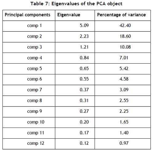
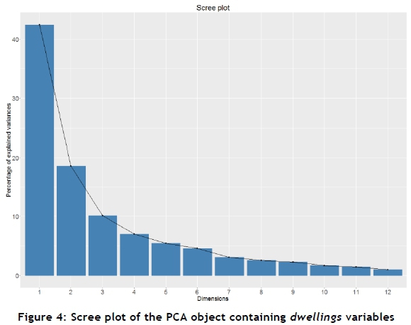
Table 7 shows the eigenvalues and percentage of variance accounted for by each of the 12 calculated principal components (PCs). The next step is to select and inspect the 'significant' components that the PCA produced. The non-quantitative method of component selection, presented by Jackson [7] and Peres-Neto et al. [14], is that of looking for a natural break between the 'large' eigenvalues and the 'small' eigenvalues, using a scree plot. The factoextra library is used to create a scree plot that is useful for visualising the variance accounted for by each principal component.

Figure 4 is a graphical representation of the components and their respective percentage of variance. A point analysis shows that the natural break in the curve appears somewhere between PC 3 and PC 4.

 

 

For a more quantitative selection method, Jackson [7] and Peres-Neto et al. [14] propose retaining the components whose eigenvalues are greater than the average of all the eigenvalues, which is 1. Based on this selection method, the PCs with an eigenvalue greater than 1 are PC 1, PC 2, and PC 3. These three principal components account for 71.08 per cent of the total variance of population data for variables relating to dwelling type. The standardised values of the original 12 variables are evaluated, based on their correlation to the three respective principal components.

These values are tabulated in Table 8. From the values in this table, non-significant correlation values are disregarded; a threshold limit is required to determine this. Several statistical tests and criteria for eigenvalue assessment are proposed by Peres-Neto et al. [15]. One of these suggests using the cut-off rule of 0.5, which Richman [17] proposes in his published study. This method is less accurate than the other more scientific methods proposed by Peres-Neto et al. [15]. However, given that this study entails an exploratory analysis of a research question rather than a set of hypotheses, this threshold will be used. Streiner and Norman [20] support the use of this method when conducting exploratory analysis.

The values above the threshold limit of 0.5 are highlighted in Table 8. Extracting these variables results in eight variables showing significance from the original 12 that were analysed. The PCA therefore reduced the set of dwelling type variables by 33.34 per cent (from 12 to 8). These eight variables are sufficiently significant in their relationship to the number of customers contained in each bin.

In the next section, these variables are used in a correlation study to test which of them account for low and high bin variance.

3.2.4 Correlation analysis

The eight variables identified in the PCA have an associated population size for each bin. This section aims to identify which of the eight variables correlate with high- and low-variance bins respectively. The variables are also fitted into a linear regression model, where bin variance is used as the predictor, and the ratio of customers per bin to population size (for each of the variables) is used as the regressor. This is to compute the goodness-of-fit of the variables and to identify variables that are significant in prediction scenarios.

A linear regression model shows the goodness-of-fit by testing the calculated p-value at a 95 per cent confidence interval. If the data fitted the model, it could be expected that there would be significant correlation between bin variance and the variables. However, when trying to identify the correlation between low- and high-variance bins and the variables, a different approach is required. The profile of increasing bin variance is shown in Figure 10. This image shows that the most extreme cases of high- and low-variance bins are found at the head and tail of the profile respectively. The further away from the two ends of the profile, the more linear the variance profile becomes. The method applied in this study therefore tests for correlation for the extreme cases of low and high variance only - which can be identified by the top and bottom 10 bins respectively. A function is therefore applied to test the correlation significance between bin variance and variable ratio⁴ for the 10 lowest- and highest-variance bins.

The population variables relating to dwelling type that have a significant correlation (p-value < 0.05) to low- and high-variance bins are identified in Section 4. The research question that asked whether this type of population category can be used to explain clustering can therefore be answered with statistically justified reasoning. Other variables within the category of dwelling type have also been identified that show varying degrees of significance in a goodness-of-fit test defined by a linear regression model. In order to validate the confidence of the findings produced by this method, a new customer data set should be used to test how robust the models are.

3.2.5 Test sample analysis

The test sample, defined in Section 2, is used to test how the results of a new data set compare with the results of the train sample. The same procedures as followed for area segmentation and cluster significance are applied; however, the parameters of the bins are kept constant to obtain comparable results - i.e., a grid of equal dimensions is applied to the sample space of the train sample. The linear regression models of the train and test samples respectively are compared, as well as the population variables that showed significance in the correlation study. The results of the test sample analysis are excluded from this article.

 

4 RESULTS

4.1 Customer profiles

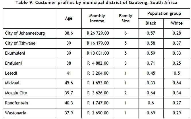
The customer profiles developed for each municipal district of Gauteng are listed in Table 9. The average customer is defined by the four variables that were selected in Section 3.

The profiles show that there is an almost directly proportional relationship between income and family size for the profiles shown. Average family size values have been rounded up or down to the nearest whole numerical value; these range from one to six across the various municipal districts. The average age spans a six-year range, and indicates that the average customer in Gauteng is middle-aged. The two primary population groups, Black and White, are shown in the profiles. However, the detailed results that include the proportions of all population groups for each profile are excluded from the results in this article. These profiles enable the retailer to align marketing campaigns based on target market characteristics as defined in this study - e.g., the average customer residing in the City of Johannesburg is likely to purchase either more expensive, better quality furniture, or furniture that caters for a large family, typically with children, while a Randfontein customer might be interested in smaller products in a more affordable price range than those that interest the City of Johannesburg customer. The data used in this study did not include product descriptions; the population group, however, might impact the style of furniture that is preferred by each customer profile.

4.2 Customer clusters

The second section of the results provides insights into customer density, shown by bins in the grid-based clustering method that was applied to the sample area. Following the regional segmentation of customer profiles (by municipal district), the same administrative boundaries are used to illustrate customer clusters by various geographical regions of Gauteng. Figure 5 shows the mean variance of the bins for each municipal district of Gauteng.

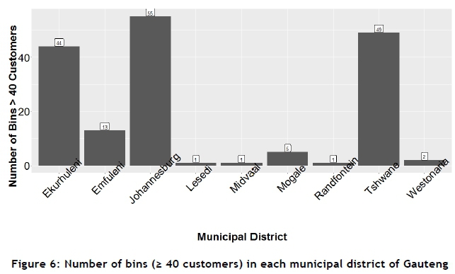
The number of bins containing more than, or equal to, 40 customers is shown in Figure 6. The train sample produced 172 bins that contain more than 40 customers from the initial 2 585 bins created by the grid-cluster method. Figures 8 and 9 show that City of Tshwane and Ekurhuleni have a lower mean value for bin variance than the City of Johannesburg, Emfuleni, and Mogale City. The remaining districts contain a negligible number of bins from which to draw comparisons.

4.2.1 Linear regression and correlation models

This section shows and discusses the results of the linear regression model that fits the values of the test and train samples respectively, and the correlation tests conducted for each sample.

Train sample

The results of the linear regression model for the train sample are shown below:

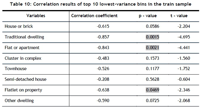
The output shows that, for the eight significant dwelling type variables selected in the PCA, the linear model passes the goodness-of-fit test at the 95 per cent confidence interval (p-value < 0.05). Three variables were found to fit the model to a significant degree: house or brick, semi-detached house, and flatlet on property. These three variables show an individual goodness-of-fit at the 95 per cent, 99 per cent, and 95 per cent confidence intervals respectively. This indicates that these three variables account for most of the variance in the linear regression model, and are indicative of the most probable dwelling types of the retailer's customers in the train sample. The variable(s) most responsible for high areas of clusters are shown in Table 10.

The results in Table 10 show that traditional dwellings, flats or apartments, and flatlet on a property have a significant correlation with low-variance bins at a 95 per cent confidence interval. These three variables are therefore the most likely dwelling types of the retailer's customers in areas where there is a significant degree of clustering.

 

5 CONCLUSION

Applying descriptive analytics using spatial data has been shown to produce insights that add strategic value to the retailer's business environment. With a specific focus on creating customer profiles and identifying densely-populated customer clusters, this study has discussed how these two objectives could be used to enhance location-based marketing campaigns in a retail sales environment. The use of geocoded customer delivery addresses, together with population data, has revealed the key attributes of customers, based on specific geographical segments in Gauteng, South Africa. The application of proven statistical methods was conducted using R. Several reproducible models were built that enabled data transformations, the handling of complex data structures, and the handling of spatial data. The study has produced a baseline of customer intelligence that can be further enhanced by overlaying the customer data with more sophisticated customer information, such as product (order) details, value of goods purchased, and detailed delivery information (dispatch information, order life cycle information, and shelf life of products).

The information delivered in this article enables the furniture retailer to increase market share, and hence profitability, by improving custom-product association and the targeted marketing of these products. Consequently, in addition to these business improvements, customer satisfaction is improved, as their needs are better understood, based on their locations.

 

REFERENCES

[1] ArcGIS. 2016. ArcGIS online help. [Online] Available at: https://doc.arcgis.com/en/arcgis-online/reference/shapefiles.htm [Accessed 27 June 2016].         [ Links ]

[2] Daniel, D. 2007. Five key business intelligence trends you need to know. [Online] Available at: http://www.cio.com/article/2437743 [Accessed: 24 June 2016].         [ Links ]

[3] ESRI. 2010. ESRI Shapefile technical description: An ESRI white paper. [Online] Available from: https://www.esri.com/library/whitepapers/pdfs/shapefile.pdf [Accessed 27 June 2016].         [ Links ]

[4] Frost & Sullivan . 2015. Customer intelligence is the new black: A Frost and Sullivan white paper. [Online] Available from: http://www.sourcingfocus.com [Accessed 27 May 2015].         [ Links ]

[5] Han, J. & Kamber, K. 2006. Data mining: Concepts and techniques, 2nd ed. San Francisco: Morgan Kaufmann Publishers.         [ Links ]

[6] Horn, X. 2016. Machine learning: Process, model validation & feature engineering. [Online] Available from: http://rusers.co/meetups/RUsersXanderHorn [Accessed 1 July 2016].         [ Links ]

[7] Jackson, D.A. 1993. Stopping rules in principal components analysis: A comparison of heuristical and statistical approaches, Ecology, 74(8), pp 2204-2214.         [ Links ]

[8] Kassambara, A. & Mundt, F. 2016. factoextra: Extract and visualize the results of multivariate data analyses. R package version 1.0.3. https://CRAN.R-project.org/package=factoextra        [ Links ]

[9] Husson, F., Josse, J. and Lê, S. 2008. FactoMineR: An R package for multivariate analysis, Journal of Statistical Software, 25(1), pp 1-18.         [ Links ]

[10] Manikandan, S. 2010. Data transformation, Journal of Pharmacol & Pharmacother, 1(2), pp 126-127.         [ Links ]

[11] Archana, R.A, Hegadi, R.S. & Manjunath, T.N. 2012. A study on sampling techniques for data testing, International Journal of Computer Science and Communication, 3(1), pp 13-16.         [ Links ]

[12] Municipal Demarcation Board. 2016. Boundary data. [Online] Available at: http://www.demarcation.org.za/index.php/downloads [Accessed 2 June 2016].         [ Links ]

[13] Pebesma, E.J. & Bivand, R.S. 2005. Classes and methods for spatial data in R. R News 5(2), http://cran.r-project.org/doc/Rnews/.         [ Links ]

[14] Jackson, D.A., Peres-Neto, P. & Somers, K.M. 2005. Stopping rules for determining the number of non-trivial axes revisited, Computational Statistics & Data Analysis, 49(4), pp 974-997.         [ Links ]

[15] Jackson, D.A., Peres-Neto, P. & Somers, K.M. 2003. Giving meaningful interpretation to ordination axes: Assessing loading significance in principal component analysis, Ecology, 84(9), pp 2347-2363.         [ Links ]

[16] R Core Team. 2016. R: A language and environment for statistical computing. Vienna, Austria: R Foundation for Statistical Computing. URL https://www.R-project.org/.         [ Links ]

[17] Richman, M.B. 1988. A cautionary note concerning a commonly applied eigen analysis procedure, Tellus, 40B(1), pp 50-58.         [ Links ]

[18] Scott, D.W. 1979. On optimal and data-based histograms, Biometrika, 66(3), pp 605-610.         [ Links ]

[19] Statistics South Africa. 2011. Living conditions survey, 2011 [dataset].         [ Links ]

[20] Streiner, D. & Norman, G.R. 2011. Correction for multiple testing, CHEST, 140(1), pp 16-18.         [ Links ]

[21] Theodorou, V. 2014. Quality measures for ETL processes. In Proceedings of the 16th International Conference on Data Warehousing and Knowledge Discovery, DaWaK 2014, edited by Ladjel Bellatreche and Mukesh K. Mohania, 9-22. Lecture Notes in Computer Science, number 8646. Munich, Germany: Springer.         [ Links ]

[22] University of Toronto. 2002. Data clustering techniques. [Online] Available at: http://www.cs.toronto.edu/~periklis/pubs/depth.pdf [Accessed 2 June 2016].         [ Links ]

[23] Vassiliadis, P. 2009. A survey of extract-transform-load technology, International Journal of Data Warehousing & Mining, 5(3), pp 1-27.         [ Links ]

[24] York University Libraries. 2016. Geospatial data. [Online] Available at: http://researchguides.library.yorku.ca/content.php?pid=245987&sid=2176375 [Accessed 1 July 2016].         [ Links ]

 

 

Submitted by authors 12 Sep 2016
Accepted for publication 2 Jul 2017
Available online 31 Aug 2017

 

 

* Corresponding author: antonie@sun.ac.za
# The author was enrolled for an M Eng (Industrial) degree in the Department of Industrial Engineering, Stellenbosch University
1 The model constructed in R that will produce spatial data insights.
2 A sufficient size of customer data need to be used to identify significant customer clusters.
3 These customers' attributes are determined by those of the ward in which they reside.
4 Ratio of customers per bin to population size per bin (for each population variable).