GENERAL ARTICLES

 

Framework for identifying the most likely successful underprivileged tertiary study bursary applicants

 

 

R. Steynberg^{*, #}; D.P. Lötter; J.H. van Vuuren

Department of Industrial Engineering, Stellenbosch University, South Africa

 

 

---

ABSTRACT

In this paper, a decision support system framework is proposed that may be used to assist a tertiary bursary provider during the process of allocating bursaries to prospective students. The system identifies those in an initial pool of applicants who are expected to be successful tertiary students, to facilitate final selection from a shortlist of candidates. The working of the system is based on various classification models for predicting whether bursary applicants will be successful in their respective tertiary studies. These model predictions are then combined in a weighted fashion to produce a final prediction for each student. In addition, a multi-criteria decision analysis method is used to assign each of the applicants to a ranking level. In this way, the system suggests both a predicted outcome for each candidate and a ranking according to which candidates may be compared. The practical working of the system is demonstrated in the context of real data provided by an industry partner, and the success rate of the system's recommendations is compared with that of the industry partner.

---

OPSOMMING

In hierdie artikel word 'n raamwerk vir 'n besluitsteunstelsel daargestel wat gebruik kan word om 'n tersiêre beursvoorsiener gedurende die beurstekenningsproses aan voornemende studente by te staan. Die stelsel identifiseer aansoekers uit 'n aanvanklike poel vir wie daar 'n verwagting bestaan dat hulle suksesvolle tersiêre studente sal wees, om sodoende die finale seleksieproses uit 'n kortlys te fasiliteer. Die werking van die stelsel berus op verskeie klassifikasiemodelle vir die voorspelling van sukses van aansoekers tydens hul voorgenome tersiêre studies. Hierdie modelvoorspellings word dan op 'n geweegde wyse gekombineer om 'n oorkoepelende voorspelling vir elke student daar te stel. Daar word ook van 'n multi-kriteria besluitnemingsmetode gebruik gemaak om elkeen van die aansoekers aan 'n rangorde vlak toe te ken. Op hierdie wyse lewer die stelsel beide 'n voorspelling aangaande die verwagte sukses van elke kandidaat en 'n ranglys waarvolgens kandidate met mekaar vergelyk kan word. Die praktiese werkbaarheid van die stelsel word aan die hand van werklike data wat deur 'n industrie-vennoot verskaf is, gedemonstreer, en die sukseskoers van die stelsel se aanbevelings word met dié van die industrie-vennoot vergelyk.

---

 

 

1 INTRODUCTION AND PROBLEM BACKGROUND

The United Nations Educational, Scientific and Cultural Organisation (UNESCO) has stated that a lack of qualified labour is one of the most important factors constraining growth and the possibility for sustainable development within a country [1]. Indeed, the quality of local tertiary education may be seen as critically important for the development of South Africa. While the quality of tertiary education is important in this sense, actually gaining access to tertiary education by having financial barriers removed is equally important, and is becoming an increasingly relevant issue if one considers the recent 'Fees Must Fall' campaign [2], a student-driven movement that was initiated in October 2015 and that aimed to remove tertiary fees for students altogether, specifically for underprivileged students.

The majority of South Africa's youth may never be able to participate in tertiary studies without financial assistance because they or their families are not able to afford it. Due to the low minimum wage in South Africa, the difference between obtaining financial assistance and not obtaining financial assistance will most likely determine the financial standing of an individual for the remainder of their life [3].

A variety of non-governmental organisations (NGOs), governmental organisations and private corporations assist underprivileged individuals in this respect by funding their tertiary studies. The research reported in this paper has been carried out in collaboration with one such NGO that provides financial support specifically to individuals from poor rural communities within South Africa.

The NGO currently uses a very basic method of weighted criteria when selecting candidates who are earmarked for financial support in the form of bursaries. Although the current process works reasonably well, it is not optimised and is very time-consuming. A need to streamline the process by means of automated decision support has been identified.

Multiple criteria decision analysis (MCDA) techniques form a subfield of operations research and other statistical learning methods. These mathematical techniques form the basis of a decision support system (DSS) framework presented in this paper. The DSS may be used by the industry partner and other similar organisations to assist their managements in the process of allocating a limited number of bursaries to applicants, based on their expected success when studying at tertiary level.

The aim of the DSS framework is not to select candidates automatically from an initial list of applicants, but rather to provide a recommendation about high-quality trade-off candidates from whom to choose, based on pre-specified criteria and parameters. The DSS assists decision-makers by decreasing the number of applicants in the initial pool in order to facilitate final selection from a shortlist of candidates.

 

2 LITERATURE REVIEW

This section contains a review of the scientific literature that is applicable to the selection problem described above. First, the concept of statistical learning is reviewed, after which a discussion is included on data partitioning and resampling during the process of statistical learning. Thereafter, five classification models are briefly described. These models form part of the DSS proposed in this paper. Next, a number of ensemble learning models are described, as well as how model weighting is fundamental to this concept. The final part of this section contains a brief discussion on the field of multi-criteria decision analysis (MCDA), and how a typical MCDA model is formulated. Finally, the outranking MCDA method of ELECTRE is highlighted because it also forms part of the DSS proposed in this paper.

2.1 Statistical learning

A relationship exists between the input variables and the output variable of a statistical process [4]. The input variables are also sometimes referred to as independent variables, whereas the output variables are also called dependent variables [5]. This relationship may be expressed mathematically as Y = f(X₁,X₂, ...,X_m), where Y represents the output variable and X₁, X₂, ... ,X_mare the input variables. The p input variables are aggregated by some function ƒ in such a manner as to predict the value of Y. 'Prediction' here refers to the process of estimating the output of a certain process with known input. The estimated output is denoted by Y.

Two stages exist during statistical learning, namely learning and validation; each of these stages requires its own data. Statistical learning models must first be taught how to 'think' during the learning phase, after which they 'apply' their knowledge during the validation stage when presented with (hitherto unseen) validation data [6].

2.2 Classification models

If the output predictions are categorical in nature, the above-mentioned process is referred to as classification. If only two output classes exist, such as 'Yes' and 'No', or '1' and '0', the process is referred to as binary classification [6]. Brief overviews of five well-established statistical learning paradigms that may be employed for the purpose of binary classification are included in this section. These paradigms are Logistic regression, Classification and regression trees (CART), Random forests, a tree-classification algorithm called C4.5, and Support vector machines (SVMs).

2.3 Logistic regression

The fundamental assumption of logistic regression is that the probability of a specific event occurring follows a logistic distribution. The probability of the desired event occurring may then be determined as

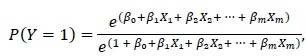
where ß₀, ß₁, ... ,ß_mare the respective coefficients of the input variables X₁, X₂, ... ,X_m. These coefficients may be estimated using the method of maximum likelihood [6].

2.4 Classification and regression trees

A classification tree is produced by growing a rooted tree, starting from the root and generating branches that form new nodes. Each node represents a specific subset of the entire sample. The root represents the entire sample, while each subsequent branching represents an if-then split condition, and the process allows for a classification of data cases according to these split conditions [7]. At each branching, the sample is partitioned so as to achieve a certain splitting criterion that maximises the purity of the two child nodes. This process is repeated for each new node in the tree until a stopping criterion is satisfied or there exists a node for each case in the data, at which point the tree is known as a maximum tree. A maximum tree results in a so-called overfit of the data, and hence it is required that such a tree be pruned back (made smaller) so as to be able to predict accurately the outcome of unseen observations [4].

According to Timofeev [8], the Gini splitting rule or Gini index is the most popular impurity function for classification trees. Let the number of dependent variable classes at some node in the CART be k and denote the total number of classes by K. Also, let the proportion of observations of class k in node t be _tk. Then the Gini splitting rule maximises

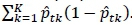
2.5 Random forests

The method of Random forests uses many trees produced during a CART-like analysis so as to obtain improved prediction ability. A bootstrapped sample is drawn from the learning set and a CART analysis is performed. During the analysis, each of the m independent variables is considered to be a possible splitting variable at each node, but in random forests only a random subset of all the variables is considered as possible splitting variables at each node. The size of this subset is typically taken as where m is the total number of independent variables present in the model [9].

The process of selecting a bootstrapped sample and splitting on only the subset of randomly selected variables at each node is repeated a predefined number of times. The resulting trees are grown to maximum size, or are bounded as specified by a minimal node size criterion. In either case, the trees are all left un-pruned. The final predictions of test observations are either the majority vote for classification trees or the average for regression trees [10].

2.6 The C4.5 algorithm

The C4.5 tree-construction algorithm, developed by Quinlan [11], is similar to CART in the sense that it starts with all the training data in a single root node and partitions it into subsequent nodes based on a particular splitting criterion. In the case of C4.5, however, the default splitting criterion is based on the so-called information gain ratio.

Similar to the pruning process of CART, the C4.5 algorithm reduces the full tree down to a simpler one so as to reduce the effect of over-fitting. New observations may be entered into the tree and, depending on the terminal node in which they are classified, are assigned an estimated outcome label [12].

2.7 Support vector machines

A SVM uses a single hyperplane to separate, according to the largest margin possible, those observations in the training set belonging to each of two different classes. The observations in the two classes located closest to the hyperplane are known as support vectors. It often happens, however, that such a hyperplane cannot be found, in which case a further step is taken by mapping the data into a higher-dimensional space, known as a feature space, with the aid of a pre-specified kernel function. Within this feature space, the hyperplane is easier to place appropriately. The outcome of new observations may then be predicted, based on which side of the hyperplane they fall [13].

2.8 Classification modelling assumptions

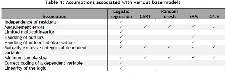
The five modelling paradigms described above are henceforth called base models. Like all statistical or machine-learning models, these base models rely on certain assumptions that have to be validated to justify their use. A brief explanation of eight fundamental assumptions applicable to the base models is provided in this section.

The assumption of independence of residuals requires that the residuals, not the raw observations themselves, be independent. If this is not the case, the residuals are said to be autocorrelated. Risk of the assumption of independence of residuals being violated is mostly of concern in the context of time series data or longitudinal data, such as stock market prices (where a stock's current price is related to that on the previous day and that on the following day). According to Ayyangar [14], one way of testing for autocorrelation involves computation of the Durbin-Watson coefficient. This coefficient falls in the range of [0, 4], where value 2 represents no autocorrelation, and a value between 1.5 and 2.5 is deemed acceptable.

As the name suggests, the assumption of measurement errors relates to errors that have infiltrated into the data during the process of collecting, observing, and/or measuring the data. These errors may cause the means of the samples to shift up or down due to the bias introduced [15].

According to Winston [16], multicollinearity exists between two or more independent variables within a multiple regression model if a positive or negative linear relationship exists between them. A well-known approach to identifying multicollinearity among independent variables involves determining the variance inflation factor (VIF) for each independent variable [17]. A VIF value of 1 indicates that no multicollinearity is present, while a value of 10 or above is typically taken as a rule-of-thumb indicating that the specific independent variable is associated with severe multicollinearity within the model.

According to Moore et al. [18], an outlier observation may be defined as "an individual value that falls outside the overall pattern". It is possible to identify outliers using a proximity matrix in conjunction with random forests.

If a data point's inclusion in or removal from a base model has a considerable impact on the model outcome, it is called an influential observation. Little and Silal [19] explain how to identify influential observations by means of Cook's distance metric, where a generally accepted cut-off value of 1 may be taken as the point above which an observation may be considered influential. Mutually exclusive categorical dependent variables imply that the two groups or classes of a dependent variable (such as Graduated and Withdrew) have to be mutually exclusive - i.e., not overlapping [20].

The minimum sample size assumption is applicable to all the base models described above. The minimum sample size requirements for CART, Random forests, SVM, and C4.5, are 240 for the smallest class, 110 in total, 60 for the smallest class, and 240 for the smallest class, respectively [21], [22]. In the context of multiple logistic regression, Peduzzi et al. [23] suggest that the minimum number of observations in a sample should be at least 10m/p, where m is the number of independent variables and p is the proportion of observations whose outcome is classified into the smallest class. Only applicable to logistic regression, the correct coding of a dependent variable requires that the desired outcome (such as Graduate) needs to be given the label '1' and the undesired outcome the label '0' [20]. According to Park [20], the linearity of the logit assumption further requires that the independent variables be linearly related to the logit transform of the dependent variable. This assumption, only applicable to quantitative variables, may be tested by means of the Box-Tidwell method [24]. This method involves including all quantitative independent variables (as only quantitative variables are applicable for this assumption), as well as the natural log transform of each quantitative independent variable in a logistic regression model. If any of the log transform variables are shown to be statistically significant, it may be assumed that the assumption of linearity of the logit has been violated.

The assumptions discussed above and the base models to which they apply are listed in Table 1.

Once predictions have been obtained from multiple base models, their predictions need to be integrated so as to facilitate a coherent decision. The process of combining the statistical predictions from multiple base models in a pre-specified manner to obtain an overall prediction is known as ensemble learning. According to Opitz and Maclin [25], Merz [26], and Dietterich [27], it has been demonstrated that the predictive ability of ensemble models is often superior to the predictive ability of any single constituent classifier base model. Ensemble models function based on the notion of exploiting the complementary strength of different learning models.

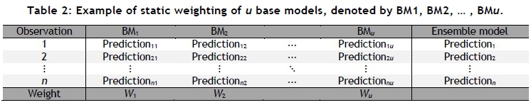
Many ensemble models require that the individual base models be weighted before being integrated. Although other types of ensemble methods exist in the literature, a brief discussion on static combination integration follows. Combination integration implies that the predictions of all the base models are considered, as opposed to only those of a single best base model. The descriptor static implies that only one weight is assigned per base model for all the alternatives, as opposed to different weightings for each alternative [28].

It is possible to produce a prediction, denoted by Prediction_nu, for each of n observations by each of u base models. Using the concept of weighting voting, it is then possible to assign a weighting to each of the , models based on their combined predictive accuracy of all the observations in the testing set, as illustrated in Table 2.

2.10 Multi-criteria decision analysis

MCDA is a well-known branch of the theory of decision-making. MCDA represents a family of methods that may be used to weigh up a number of possible choices or alternatives in the presence of various, possibly conflicting, decision criteria or objectives, in search of solutions that embody suitable confliction trade-offs [29].

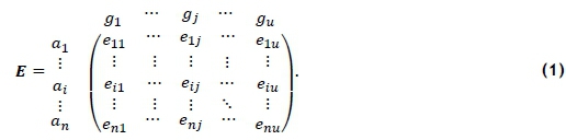
According to Mota et al. [30], an MCDA problem may be formulated as follows. Let A = a₁, ... ,a_n denote the set of possible alternatives when analysing a discrete decision space. The alternatives or possible actions are the available options from which a decision-maker may wish to select a certain number in a specific manner. Let G = g₁... ,g_udenote the set of criteria (or attributes) relevant to the decision at hand. Each of the n criteria represents a dimension in which an alternative may be evaluated. A score e_ij- may be assigned by the decision-maker to alternative i according to criterion j which is indicative of how well that alternative performs in the context of criterion j. These scores together form an u ₓ n evaluation table or performance matrix

One of three main categories into which MCDA methods may be classified is known as outranking models. In outranking models, various alternative courses of action, or alternatives, are compared in a pairwise manner so as to determine the extent to which the selection or preference of one action over another may be affirmed. By combining the information collected on these preferences, for all criteria involved, outranking models determine the strength of evidence favouring one alternative above another. Outranking models do, however, not produce a value function indicating the extent to which one alternative is worse than its predecessor or better than its successor in the resulting ranking [31].

The ELimination Et Choix Traduisant la REalite (ELECTRE) methods are a family of outranking MCDA methods. The first member of the family, ELECTRE I, was initially proposed in 1965; the other methods have since joined the family. A very popular and widely employed ELECTRE ranking method, known as ELECTRE III, is briefly described in closing this section [32].

Figueira et al. [33] explain that ELECTRE III relies on the concepts of concordance and non-discordance, since by these notions it is possible to test the outranking relation allegation, 'a outranks b', for acceptance. The principle of concordance requires that a majority of the n criteria, with their relative weightings taken into consideration, should be in favour of an allegation in order for it to be valid. The second principle, non-discordance, states that the allegation may be deemed valid provided that none of the criteria which form part of the minority strongly oppose the assertion.

By combining these two principles, the formation of a credibility index is made possible, by which the credibility of the allegation 'a outranks b' is quantified for each possible pair of alternatives. Thereafter, a process of distillation follows, during which a qualification of each alternative is constructed. The qualification of alternative is calculated as the number of alternatives that outranks, less the number that outrank . Once the processes of ascending distillation and descending distillation have been completed, the two rankings may then be combined to form the final ranking of alternatives by placing them on rank levels [32].

 

3 FRAMEWORK FOR COMBINING STATISTICAL LEARNING AND MCDA

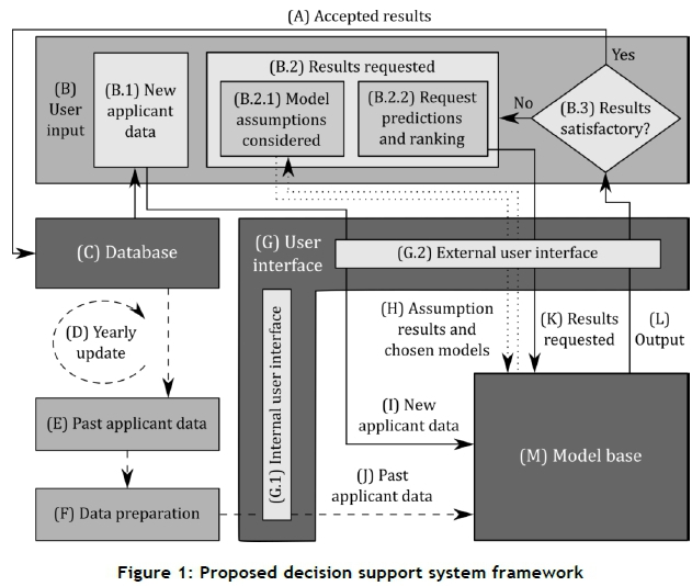
The DSS framework proposed in this paper for ranking bursary applicants is shown graphically in Figure 1. Doucet [34] states that a DSS in general consists of three main components, namely a database, a model base, and a user interface. These three components indeed form the basis of our framework, and are denoted by (C), (G), and (M), respectively, in Figure 1.

A database allows for the structured storage of related data, from where it is accessible to the other components of the DSS. Human-computer interaction (HCI) is made possible by what is known as a user interface or graphical user interface (GUI). It provides a link between the human operator and the computerised decision support system, allowing users to interact with the system. The user typically provides all the inputs required by the system and obtains all the relevant outputs via this GUI. The model base component contains the models used to solve the problem at hand and present different alternatives for the decision-making process. Such a model base may materialise in various forms, such as single mathematical algorithms or optimisation techniques. In other cases, the model base may be a combination of various algorithms, techniques, or methods [35].

Two main activities occur within our framework in Figure 1. First, the model base (M) requests past applicant data (J) so that model learning may take place, indicated by the dashed lines. This is performed by receiving the past applicant data (E) from the database (C), and then preparing the data (F). Data preparation involves cleaning the data of any major faults and ensuring that it is in the correct format. The cleaned past applicant data may then be passed to the model base.

The second main activity is concerned with the input that the user may provide to the system (B). The user may request results (B.2) from the model base (M) in the form of predictions and/or rankings of students (B.2.2) upon providing the model base (M) with new applicant data (B.1). The results requested by the user (K) also contain information on the specific dependent and independent variables the user prefers. The first task performed by the model base (M) is to evaluate the assumptions of the data and models within the model base, indicated by the dotted line. The results of the assumption evaluation are passed to the user (H), who considers the results (B.2.1) and is able to select which models within the model base he/she would still like to have activated, despite possible assumption violations that may exist for those models. The model base (M) is then passed to the selected base models (H). Using the activated base models (H) and their training in the context of past applicant data (J), the model base (M) produces results for the new applicants (I) and presents them to the user (L). The user may then consider them (B.3) and, if found to be satisfactory, they may be accepted and passed (A) to the database (C). Alternatively, if found to be unsatisfactory, the user may request new results.

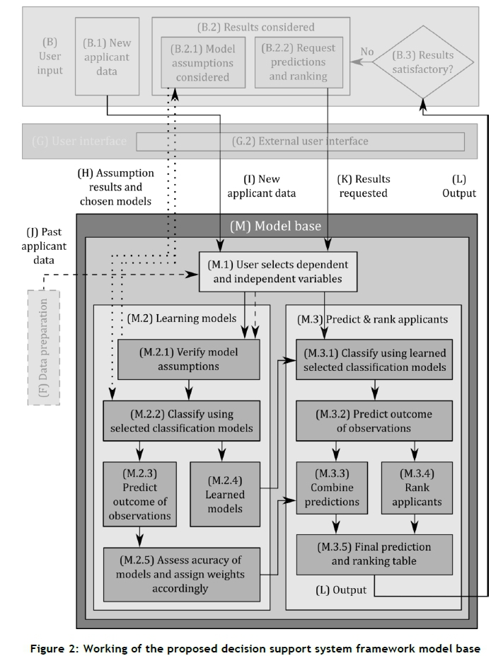
The processes followed within the model base (M) are further shown in Figure 2, the workings of which are as follows. As mentioned above, the user requests predictions and/or rankings of new applicants (B.2.2) by providing data of the new applicants (B.1) and selecting dependent and independent variables to be used during the analysis. All these preferences and data are accumulated in block (M.1), which also receives the cleaned past applicant data (J). The remainder of the model base is partitioned into the processes of learning (M.2), and predicting outcomes and ranking applicants (M.3).

First, the process of learning involves evaluating the data and model assumptions, and passing the results back to the user (H), who may then select the final models to be used. All of the past applicant data (J) may be used to learn in the selected classification modelling paradigms (M.2.2). At this point the classification models may be considered taught (M.2.4). The outcome of the validation set of students may then be predicted (M.2.3). By assessing the predictive accuracy of each classification base model, static weights may be assigned to them.

The process of predicting the outcome and ranking new applicants (M.3) occurs as follows. The learned models (M.2.4), new applicant data (M.1), selected dependent and independent variables (M.1), and selected classification base models (M.3.1) are used to predict the outcome of the new applicants (M.3.2). Thereafter, using the model weights (M.2.5), the base model predictions of the new applicants are combined so as to produce a single prediction for each applicant (M.3.3).

By studying the static combined weighting (illustrated in Table 2) and an appropriate MCDA model, such as the one illustrated in (1), it should be evident that many similarities exist between the formats of the two. An outranking MCDA method is applied to rank the applicants into rank levels. Applicants are considered as the alternatives, the different classification models (M.3.1) as criteria, the predictions of the models as the criterion scores, and the base model weightings (M.2.5) as the criteria weights. It is then possible to rank the new applicants (M.3.4) in an appropriate manner so as to produce rank levels for each. A final table containing both the prediction and ranking of each new applicant may then be formed and produced as output (L) to be considered by the user (B.3).

 

4 CASE STUDY

In this section, we employ the DSS described above to perform a case study analysis on data provided by the industry partner alluded to in §1. First, the data are analysed. The various available data fields are presented and briefly discussed next. Thereafter, the data are cleaned and prepared so that they are adequate for use as input into the DSS. This is followed by a description of the process of selecting the dependent and independent variables for the case study. The working of the proposed DSS is then demonstrated by referring to the user interface of an implementation of the DSS framework of §3 in the context of the case study at hand. Finally, the results of the case study are discussed in some detail.

4.1 Available sample

A data sample of 1 445 underprivileged South African tertiary students who have previously received funding from the industry partner was collected for analysis purposes. The students started their tertiary studies between 2006 and 2014, and all of them have either successfully obtained their qualifications or withdrawn. As indicated in block (F) of Figure 1, the next step was to prepare the data for analysis, as explained next.

4.2 Data fields

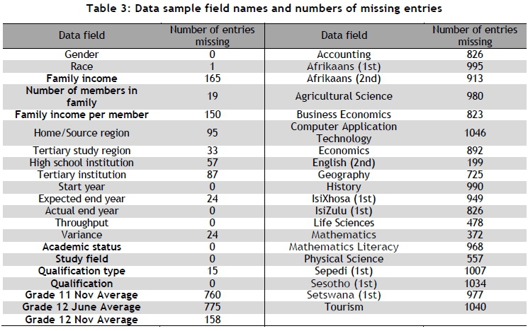
The 41 data fields of the data sample, as well as the number of entries missing from each field, are shown in Table 3. An explanation of the variables of interest for this paper now follows.

Family income indicates the total income of the family of which the applicant is a member, while Number of members in family indicates the size of that family (the number of people supported by the family income). The field Family income per member refers to the average income per family member of the household from which the student originates, and may be calculated by dividing the family income by the number of members in the family.

The Academic status field indicates the student's current academic status. A student is assigned one of two academic statuses: either Graduated or Withdrawn. 'Graduated' indicates that the student has successfully completed his or her tertiary degree. 'Withdrawn' indicates that a student has withdrawn from his or her tertiary studies.

Study field refers to the academic field of the student's intended tertiary studies, such as Arts, Commerce, Education, Science, Engineering, or Medical. The Qualification type field indicates the type of qualification the student either attempted or obtained. The three types of qualification types are Degree, Extended degree, and National Diploma.

The Qualification of a student refers to the exact qualification he or she attempted or obtained (e.g., BSc Chemical Science or Diploma of Graphic Design). There are 194 different qualifications in the sample.

Grade 11 Nov Average, Grade 12 June Average, and Grade 12 Nov Average are the average marks obtained by a student for each of those exams. Finally, the twenty school subjects taken by at least 55 of the students are listed.

4.3 Data cleaning

The cleaning of the data involved removing or correcting any erroneous values. A total of 319 values were identified as erroneous and corrected if possible, or else removed. In cases of removal, only the specific values were removed (not the entire data record or entry relating to that student). In addition, over the time period related to the sample, many name changes and merges of tertiary institutions took place, and thus it was necessary to update all the tertiary institution names to reflect their most recent names.

4.4 Dependent and independent variables

For the purpose of this study, the dependent variable was chosen so that those students who graduated successfully from their respective tertiary institutions could be identified. The Academic status of a student was therefore chosen as the dependent variable. Those students in the sample data with the academic status of Graduated were considered academically successful, and so were assigned the label '1' for the dependent variable. All of the remaining students had an academic status of Withdrew, but only those who withdrew due to poor academics were assigned the label '0'. The term Withdrew does not necessarily refer to a student withdrawing from tertiary studies, but rather to the withdrawal of financial support from the student due to their poor academic performance. In such cases, those students may already have been excluded by the tertiary institution due to their poor academic performance, and in other instances the student may have been permitted to continue by the tertiary institutions, but could not due to lack of financial support. The NGO will thus only do this when they feel confident that the student will not complete their studies. The remaining students who withdrew for non-academic reasons, such as medical reasons or postponement of studies, were removed from the sample. Once the students who did not have one of the correct dependent variable labels had been removed from the sample, only 1 101 students remained within the sample.

In order to demonstrate the flexibility of the DSS framework, all of the remaining variables listed in Table 3 are made available as possible independent variables. The only variable listed in Table 3 that may not be considered as an independent variable is Academic status.

4.5 User interface walkthrough

The working of the DSS proposed in this paper is demonstrated in this section by referring to actual data of the case study in a walkthrough manner.

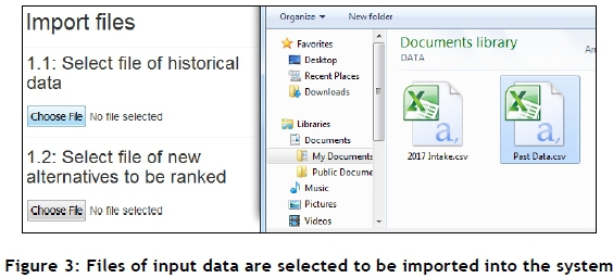
On the first screen of the GUI, the user is prompted to select two files to be imported. The first should contain past data from which the system will learn, and the second should contain data of new alternatives for which the output is not known, but desired. The column names or fields of the two files should be identical. A screenshot showing the process of selecting these two files may be seen in Figure 3. The GUI acknowledges once the two files have successfully been uploaded, after which the user may select the 'Proceed' option to proceed to the next screen.

 

 

On the next screen, shown in Figure 4, the user is required to provide three inputs. First, the user must select only one field to be used as the unique identifier of alternatives for the remainder of the analysis. Secondly, the user may select multiple fields to be used as the independent variables or input variables for the analysis. Finally, the user may select a single binary field to be used as the dependent variable or output variable. To assist the user, the system only provides those fields that are viable options for each of the three specific inputs. For the case study at hand, the MyID column was selected as the unique identifier of the students and, as discussed above, the Academic status of a student was selected to be the binary output variable. Five independent variables were then selected, namely Institution, Study field, Qualification type, Grade 12 Nov average, and Family income per member.

Once the user is satisfied with his or her selection, the 'Proceed' button may be clicked to proceed to the next screen. On each of the following screens, the user may at any point return to the previous screen, start from the first screen again, or proceed to the next screen, if applicable.

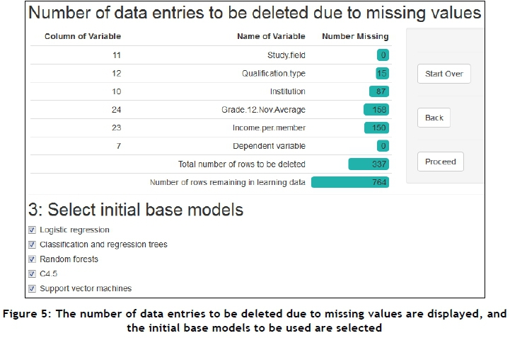
On the third screen, shown in Figure 5, the number of entries, observations or alternatives to be deleted due to missing values in any of the fields or columns selected on the previous screen are displayed in tabular form. The total number of observations deleted from the training data thus depends on the selection of variables on the second screen. In addition, the base models currently available in the DSS are listed, and the user can select those that he or she would like to include in the analysis. Note that these five models are not considered the best five models; they are merely five models from the literature known to perform classification adequately, and thus will suffice in allowing the fundamental concepts of the DSS to be showcased. For the current case study, we selected all of the available base models (the five described in §2). As before, the user may select the 'Proceed' button to proceed to the next screen.

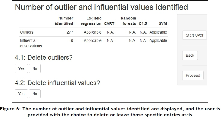
The validity of various assumptions related to the data and base models may now be assessed. On the next screen, depicted in Figure 6, the user is presented with the number of outliers and influential observations that were identified in the training data, and to which of the base models selected on the previous page they are applicable. The user may then select whether or not to delete the outliers (4.1) and influential observations (4.2). For the case study at hand, let us assume that the user felt that too large a percentage of the observations left in the training data would be removed if the outliers were to be deleted.

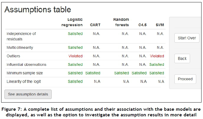
Once the user has made his or her choice, the 'Proceed' button may be clicked to proceed to the next screen, shown in Figure 7, where the user is presented with a list of all assumptions applicable to each of the base models selected, and whether these assumptions are satisfied or violated. Note that the assumption of outliers is violated in the context of the case study, since the outliers were not removed on the previous screen.

If the user desires to study further details on the assumptions, he or she may click the 'See assumption details' button, upon which the exact values determined for each assumption are shown, as depicted in Figures 8-11.

More specifically, the Durbin-Watson coefficient value for the independence of residuals, the VIF scores for each of the independent variables (each category of a qualitative variable becomes a variable for this assessment), the number of outliers and influential observations identified (as on the previous screen), the minimum sample size requirements of the different base models, and the linearity of the logit outcome for each quantitative and ordinal variable are displayed.

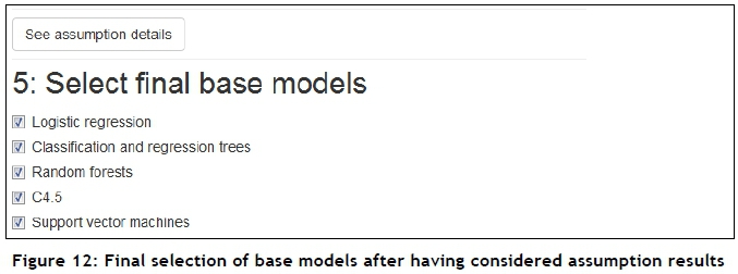
Once the user has assessed the assumption details, he or she may click the 'Back' button to return to the previous screen, displayed in Figure 12. Armed with the knowledge of the assumption assessment results, the user may then make his or her final selections of which of the base models should be used for the analysis. In this way, the user is placed in control, but is also made aware of the potential risks associated with his or her choices. In the case of the current case study, we chose to take the risk associated with retaining the outliers and still selecting both the Logistic regression and Support vector machine base models along with the other three base models, as shown in Figure 12. As before, the user may again select the 'Proceed' button to proceed to the next page.

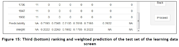
The system is now ready to predict the outcome for and rank each of the alternatives in the test set of the learning data. To achieve this, the system performs two operations. First, based on the predictive accuracy of each base model, each model is assigned a weight, which is used to produce the single weighted vote for each alternative (student). In addition, an MCDA outranking method, in this case ELECTRE III, is used to place each alternative on a ranking level. Eleven rank levels were identified in the case study.

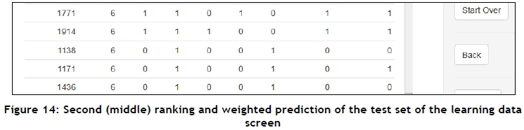
The results of the process described above may be seen in Figures 13-15. The weighted prediction for each alternative is shown in the second-last column, and the rank level of each alternative in the second column. The predictability and weight for each of the base models for the case study may be seen in Figure 15. Note that the predictability of the weighted prediction, of 76%, is higher than any of the single base models' predictability. Also, notice that at some point there is a partition of the 1 's and 0's of the weighted predictions. In this case, as may be seen in Figure 14, the partition occurs within rank six. The user may yet again select 'Proceed' to continue to the next screen.

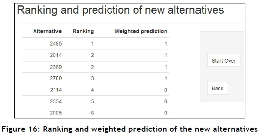
The system is now ready to perform its final operation - to predict the outcome for and ranking of the new alternatives, for whom the corresponding output is not known, contained in a new data set. The new data set has identical fields to those of the historical set. The selected base models, which have been trained according to the learning data, now make predictions for the new data. The predictions from the various base models are combined using the weightings of the base models determined during the learning process. Finally, each new alternative is also assigned to a rank level using an MCDA outranking method - again, ELECTRE III in this case. This final prediction and ranking of the new alternatives may be seen in Figure 16.

 

 

4.6 Discussion of case study results and system capabilities

In order to consider the proposed system a success, it should satisfy at least the following three criteria:

1. First, the system should achieve a better accuracy rate than the industry partner has achieved using its current manual methods.

2. Secondly, the combined weighted prediction of a student's success should achieve a higher accuracy than any of the single base models the majority of the time.

3. Thirdly, the ranking of the students should make logical sense, and agree with the predicted outcome of the students.

The purpose of the case study presented here was to demonstrate the working of the proposed DSS in a single realistic scenario. In order to assess the performance of the system in the context of the above criteria, however, it was necessary to analyse its performance in the context of multiple different scenarios. These scenarios were generated as follows.

For each of the scenarios, the same sample set of learning data was used, as provided by the industry partner. Also, for each scenario the same dependent variable was used, namely the Academic status of the students. Four different groups of independent variables were, however, selected. Some of the variables of the four groups overlap.

The variables of the first scenario were Study field, Number of members in the family, Source region, Course length, and Qualification type. Those in the second group were Study field, Qualification type, Institution, Grade 12 Nov average, and Income per member. Those in the third were Number of members in family, Income per member, Study field, Institution, Course length, Qualification type, Grade 12 Nov average, English second language, Race, and Gender. Finally, the variables in the fourth group were Study region, Income per member, Study field, Grade 12 Nov average, and English second language.

The data provided by the industry partner (the learning data) were partitioned into two different sets for each test run: first, into a training set (used by the system to teach itself) that randomly consists of between 80% and 85% of the learning data; and next, into a testing set or test set (used by the system to test its newly taught models against predictive accuracy) that contains the remainder of the learning set. The size of these two subsets, and the specific entries contained within each, was randomised 100 times for each of the above four main scenarios (specific independent variable combinations). In this way, 400 different test runs were created for system assessment purposes.

After the 400 test runs of the DSS had been carried out, it was found that the average combined prediction accuracy of the system on the test set was 66.4%. Of the 1 101 students who remained in the sample after data cleaning, and who had received bursaries from the industry partner over the past nine years, 643 successfully graduated, while 458 were unsuccessful. This would imply a prediction accuracy of 58.4% for the industry partner. The industry partner provides bursaries with a reasonable expectation that the students will go on to graduate. It may thus be concluded that the first of the three above-mentioned criteria is satisfied, as the proposed system does produce better results than past manual attempts.

It would, of course, be possible to improve this accuracy by using a better combination of independent variables, although the ones chosen are believed to be of reasonable predictive ability. It should also be noted that, when the same analysis was to be repeated after having removed the outliers, the predictive accuracy exceeded 90%, on average. This, however, was not done, as the results thus produced would not have been appropriate for comparison with the industry partner's accuracy.

Besides the above-mentioned independent variables, many others may also produce fruitful results; but the availably of such variables is the inhibiting factor. These variables may include variables dedicated to student's family situation, number of tertiary graduates within the student's family, and other 'soft' variables such as the grit level of the student.

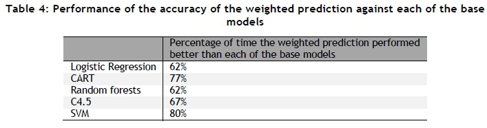
The performance of the combined weighted prediction accuracy against the individual base models, averaged over the 400 runs, may be seen in Table 4. The percentages displayed in the table were calculated by first excluding those cases for which the accuracy of the weighted prediction equalled that of a specific base model. Thus the percentages only reflect occurrences for which the weighted prediction performed strictly better than all the base models individually.

From Table 4 it is evident that the accuracy of the weighted predictions produced by the system outperforms each of the base models more than half the time. It may thus be concluded that the weighted predictions of the system are a better predictor than any of the individual base models; and so the second of the above three criteria is also satisfied.

The third criterion requires that the ranking produced by the system be logical and agree with the weighted predictions. As was shown in Figures 14 and 16, if moving in descending order down the rank levels, the predictions change from 1's to 0's at some point. This might happen within a single rank level. This phenomenon occurred for each of the 400 test runs, and makes logical sense, since the higher-ranked students should be assigned a desired outcome, and at some point down the ranking the students should be labelled as higher risks. In addition, the 76.32% average accuracy of the system's predictions indicates that the predictions and rankings that correspond to the predications may be considered accurate estimations. The third criterion may therefore also be considered satisfied.

 

5 CONCLUSION

The aim of this paper was to present a DSS framework that may be used to assist tertiary bursary providers in managing the process of allocating bursaries to prospective students. The proposed system decreases the number of applicants in an initial pool so as to facilitate final selection from the shortened list of candidates.

A brief literature review was presented, covering the core concepts related to the study. These included various fundamentals of statistical learning, as well as the working and assumptions of five classification base models, namely logistic regression, CART, random forests, the tree building algorithm C4.5, and SVMs. The remainder of the literature section was devoted to a discussion of ensemble models and MCDA models, specifically focusing on ELECTRE III.

The proposed DSS was presented next. In order to demonstrate practically its working and capabilities, data provided by an industry partner were used to perform a walkthrough demonstration of the DSS GUI. The case study presented for the demonstration purposes was a single test run for a single scenario. Results of four scenarios for 400 test runs were also averaged to demonstrate that the system satisfies three reasonable criteria required for the system to be deemed successful.

The industry partner has expressed its satisfaction with the DSS, and the head of programme development, research, and advocacy of the industry partner provided the following feedback after a presentation of the work at the industry partner's head office:

"I have found the work and presentations enormously interesting and thought-provoking ... prediction for success for Higher Education students - is not only of importance to our company, but for the whole Higher Education sector and institutions funding students. In a context that broadens access and has limited resources such tools are, I believe, vital for decision making."

 

REFERENCES

[1] UNESCO. 2015. Introducing UNESCO [Online] [Cited February 10th, 2015]. Available from http://en.unesco.org/about-us/introducing-unesco.         [ Links ]

[2] Msila, V. 2016. #FeesMustFall is just the start of change [Online] [Cited March 31st, 2016]. Available from Mail and Guardian, Jan 21. http://mg.co.za/article/2016-01-20-fees-are-just-the-start-of-change        [ Links ]

[3] De Lannoy, A., Leibbrandt M. & Frame, E. 2015. A focus on youth: An opportunity to disrupt the intergenerational transmission of poverty. South African Child Gauge, Unversity of Cape Town.         [ Links ]

[4] Hastie, T., Tibshirani, R. & Friedman, J. 2009. The elements of statistical learning. New York: Springer.         [ Links ]

[5] Draper, N. & Smith, H. 1996. Applied regression analysis. New York: John Wiley & Sons.         [ Links ]

[6] James, G., Witten, D., Hastie, T. & Tibshirani, R. 2013. An introduction to statistical learning. New York: Springer.         [ Links ]

[7] StatSoft Inc. 2016. Popular decision tree: Classification and regression trees (CART) [Online] [Cited February 3rd, 2016]. Available from http://www.statsoft.com/Textbook/Classification-and-Regression-Trees.         [ Links ]

[8] Timofeev, R. 2004. Classification and regression trees (CART) theory and applications. PhD dissertation, Humboldt University, Berlin: Center of Applied Statistics and Economics.         [ Links ]

[9] Shi, Y. & Song, L. 2015. Spatial downscaling of monthly TRMM precipitation based on EVI and other geospatial variables over the Tibetan plateau from 2001 to 2012. Mountain Research and Development 35(2), pp. 180-194.         [ Links ]

[10] Moisen, G.G. 2008. Classification and regression trees. Encyclopedia of Ecology, pp. 582-588.         [ Links ]

[11] Quinlan, J.R. 1993. C4.5: Programs for machine learning. San Francisco: Morgan Kaufmann Publishers.         [ Links ]

[12] Ruggieri, S. 2002. Efficient C4.5 [classification algorithm], IEEE Transactions on Knowledge and Data Engineering, 14(2), pp. 438-444.         [ Links ]

[13] Cortes, C. & Vapnik, V. 1995. Support-vector networks. Machine Learning 20(3), pp. 273-297.         [ Links ]

[14] Ayyangar, L. 2007. Skewness, multicollinearity, heteroskedasticity - You name it. Proceedings of the SAS Global Forum, Menlo Park (NJ), pp. 1-7.         [ Links ]

[15] Trochim, W. 2006. Measurement error [Online] [Cited October 20th, 2015]. Available from http://www.socialresearchmethods.net/kb/measerr.php.         [ Links ]

[16] Winston, W.L. 2004. Operations research: Applications and algorithms. Belmont: Brooks Cole.         [ Links ]

[17] O'Brien, R. 2007. A caution regarding rules of thumb for variance inflation factors. Quality & Quantity 41(5), pp. 673-690.         [ Links ]

[18] Moore, D., McCabe, G. & Bruce, C. 2009. Introduction to the practice of statistics. New York: W.H. Freeman and Company.         [ Links ]

[19] Little, F. & Silal, S. 2014. Risk factor response analysis. Cape Town: University of Cape Town Departments of Public Health and Statistical Sciences, pp. 1-103.         [ Links ]

[20] Park, H.A. 2013. An introduction to logistic regression: From basic concepts to interpretation with particular attention to nursing domain. Journal of Korean Academy of Nursing 43(2), pp. 154-164.         [ Links ]

[21] Li, C., Wang, J., Wang, L., Hu, L. & Gong, P. 2014. Comparison of classification algorithms and training sample sizes in urban land classification with Landsat thematic mapper imagery. Remote Sensing 6(2), pp. 964-983.         [ Links ]

[22] Cutler, D.R., Edwards, T.C., Beard, K.H., Cutler, A., Hess, K.T., Gibson, J. & Lawler, J.J. 2008. Random forests for classification in ecology. Ecology 88(11), pp. 2783-2792.         [ Links ]

[23] Peduzzi, P., Concato, J., Kemper, E., Holford, T.R. & Feinstein, A.R. 1996. A simulation study of the number of events per variable in logistic regression analysis. Journal of Clinical Epidemiology 49(12), pp. 1373-1379.         [ Links ]

[24] Hilbe, J. 2009. Logistic regression models. Boca Raton: Chapman & Hall.         [ Links ]

[25] Opitz, D. & Maclin, R. 1999. Popular ensemble methods: An empirical study. Journal of Artificial Intelligence Research 11, pp. 169-198.         [ Links ]

[26] Merz, C.J. 1998. Classification and regression by combining models. PhD dissertation. Irvine: University of California.         [ Links ]

[27] Dietterich, T. 2007. Ensemble methods in machine learning. Corvallis: Oregon State University.         [ Links ]

[28] Puuronen, S., Terziyan, V.Y. & Tsymbal, A. 1999. A dynamic integration algorithm for an ensemble of classifiers. Proceedings of the 11th International Symposium on Foundations of Intelligent Systems. London: Springer, pp. 592-600.         [ Links ]

[29] Colson, G. & de Bruyn, C. 1989. Models and methods in multiple objectives decision making. Mathematical and Computer Modelling 12(10-11), pp. 1201-1211.         [ Links ]

[30] Mota, P., Campos, A.R. & Neves-Silva, R. 2013. First look at MCDM: Choosing a decision method. Advances in Smart Systems Research 3(2), pp. 25-30.         [ Links ]

[31] Belton, S. & Stewart, T.S. 2002. Multiple criteria decision analysis: An integrated approach. Norwell: Kluwer Academic Publishers.         [ Links ]

[32] Majdi, I. 2013. Comparative evaluation of PROMETHEE and ELECTRE with application to sustainability assessment. PhD dissertation. Montreal: Concordia Institute for Information Systems Engineering (CIISE), Concordia University.         [ Links ]

[33] Figueira, J.R., Mousseau, V. & Roy, B. 2016. ELECTRE Methods. In Multiple criteria decision analysis: State of the art surveys, pp. 155-185. New York: Springer.         [ Links ]

[34] Doucet, J. 2009. Components, purpose and function of information systems [Online] [Cited October 13th, 2015]. Available from http://jennadoucet.wordpress.com/2010/03/14/components-purpose-and-function-of-information-systems/.         [ Links ]

[35] Kendall, K.E. & Kendall, J.E. 2011. Systems analysis and design. Upper Saddle River: Pearson.         [ Links ]

 

 

Submitted by authors 1 Dec 2016
Accepted for publication 12 Jul 2017
Available online 31 Aug 2017

 

 

* Corresponding author: reniersteynberg@gmail.com
# Author was enrolled for an M Eng (Industrial) degree in the Department of Industrial Engineering, Stellenbosch University