


Serviços Personalizados
Artigo
 Inglês (pdf)
 Artigo em XML
 Referências do artigo
Indicadores

Links relacionados
-
 Citado por Google
 -
 Similares em Google
Compartilhar

 Permalink
South African Journal of Industrial Engineering
versão On-line ISSN 2224-7890
versão impressa ISSN 1012-277X
S. Afr. J. Ind. Eng. vol.28 no.1 Pretoria Mai. 2017
http://dx.doi.org/10.7166/28-1-1615
CASE STUDIES
A multi-objective approach to the assignment of stock keeping units to unidirectional picking lines
Department of Logistics, University of Stellenbosch, South Africa
ABSTRACT
An order picking system in a distribution centre consisting of parallel unidirectional picking lines is considered. The objectives are to minimise the walking distance of the pickers, the largest volume of stock on a picking line over all picking lines, the number of small packages, and the total penalty incurred for late distributions. The problem is formulated as a multi-objective multiple knapsack problem that is not solvable in a realistic time. Population-based algorithms, including the artificial bee colony algorithm and the genetic algorithm, are also implemented. The results obtained from all algorithms indicate a substantial improvement on all objectives relative to historical assignments. The genetic algorithm delivers the best performance.
OPSOMMING
'n Stelsel vir die opmaak van bestellings bestaande uit parallelle eenrigting uitsoeklyne in 'n distribusiesentrum word beskou. Die doelwitte is om die loopafstand van die werkers, die grootste volume van voorraad op 'n uitsoeklyn oor alle uitsoeklyne, die aantal klein pakkette, en die totale koste van laat distribusies te minimeer. Die probleem word geformuleer as 'n meerdoelige veelvuldige rugsakprobleem, maar kan nie in 'n realistiese tyd opgelos word nie. Bevolking-gebaseerde algoritmes, insluitend die kunsmatige by-kolonie-algoritme en genetiese algoritme, is ook geïmplementeer. Al die algoritmes verkry 'n beduidende verbetering op historiese toewysings vir al die doelwitte. Die genetiese algoritme vaar die beste.
1 INTRODUCTION
The supply chain of Pep Stores Ltd (PEP) is investigated in this study. PEP is the largest single-brand retailer in Africa [15], and sells mainly clothing and footwear, with operations in more than 1,870 retail stores in Southern Africa. They have three distribution centres (DCs) and 13 transport hubs in South Africa, with a total area of more than 250,000 m2. They employ more than 15,000 people at their central offices and stores, are situated in nearly every town and village in South Africa [4]. They sell affordable merchandise and therefore have a low profit margin. To maintain their current customer base or their target market of low- to middle-income groups, items need to have constantly low markups. Each year PEP sends more than 600 million items to their stores, with more than 250 million customer transactions being conducted [15].
Products are transported in bulk from various suppliers and factories to PEP's three DCs where they are collected and packed into boxes. These boxes are then transferred to hubs to be distributed to their respective retail stores. The quantity of each product to be sent to each store is determined by the planning department at their central office to ensure that the same techniques are applied during the decision process. About half of the products sold by PEP follow a replenishment cycle, while the other half are seasonal due to changing fashion trends. PEP makes use of a push system in which seasonal stock is picked from picking lines [1]. The demand at each store is forecasted every week to avoid the cost of keeping stock in inventory, since PEP tries to minimise their storage space to allow for more items to be displayed in the stores.
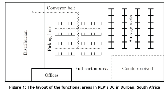
All products sold by PEP are distributed from its three DCs, located in Kuilsriver, Durban, and Johannesburg, South Africa. The DC considered in this study is the one situated in Durban, due to its high rate of processing goods and its operational flexibility compared with the other two DCs. This is attributed to the fact that most of PEP's suppliers are located in the Far East. The mathematical formulations and algorithms in this study may, however, still be applied to the other DCs, with an arbitrary number of picking lines and locations within a picking line, due to the DCs' similar order picking principles. PEP's DC in Durban is their largest, with a total area of more than 50,000 m2 [1]. The layout of PEP's Durban DC is shown in Figure 1.
Stock arrives from the suppliers in cartons at the 'goods received' area, after which it is transported either to the storage racks or to the full carton area. The storage racks store cartons that need to be repackaged into smaller cartons by assigning them to picking lines. A carton that already contains the orders of a specific store is classified as a full carton, sent to the full carton area, and directly transported to the distribution area to be shipped to the corresponding retail outlet. Once all necessary administration of a distribution (DBN) placed on the storage racks has been completed, the DBN is released to the DC and is available to be assigned to a picking line. Each DBN has an out-of-DC date - typically less than seven days from its release date - before it has to be picked from a picking line to be delivered to all retail outlets requiring the stock keeping units (SKUs) in that DBN.
Order picking is the process by which appropriate quantities of SKUs are retrieved from picking line locations by pickers moving in a clockwise direction. A picking line consists of a fixed number of locations, with a conveyor belt that leads to the distribution area, where the cartons are collected for shipping to various retail stores. DBNs consist of one or more different SKUs. A DBN consists of the same product, and each SKU in a DBN contains a different size of that product. The central planning department determines which SKUs are placed in which DBNs, and how many of each SKU are placed in a store's order. A DBN is assigned to a specific wave1 of picking, with each SKU in the DBN assigned to a specific location in that picking line - i.e., η SKUs in a DBN will take up η locations in a picking line. Thus all the SKUs in a DBN are picked in the same wave so that stores will receive different sizes of the same product at the same time. Furthermore, packages should preferably be smaller than roughly the size of a shoebox (0.006 m3) to avoid unnecessary transport and handling cost during distribution to stores. Order picking is a labour-intensive task in DCs, and accounts for approximately 55 per cent of all operating costs in a DC [1].
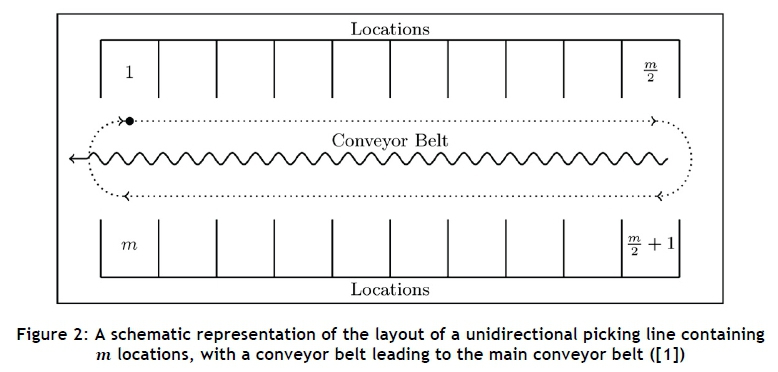
Figure 2 contains a schematic representation of the layout of a picking line in the Durban DC. Each picking line considered in this study has 56 locations (28 locations on either side of the conveyor belt). Each location can hold a maximum of five pallets of the same SKU, with the dimensions of each pallet being approximately 1 m χ 1.2 m χ 0.14 m. The dotted arrows in the figure indicate the clockwise direction in which pickers walk around the conveyor belt to collect SKUs from their assigned locations. An order contains only SKUs from a single wave of picking; thus an order exists only for a fixed wave of picking. Only when the wave of picking has been completed, may a picker move to another picking line to start another wave of picking. A store may thus have multiple orders at a given time, with each order being picked in a separate wave of picking. The Durban DC contains 12 picking lines in total, with six picking lines on either side of a main conveyor. All picking lines are situated next to one another at floor level. Order picking, populating SKUs on the picking lines, and cleaning up leftover stock all take place simultaneously on different lines. Therefore, two to four picking lines are usually available to which SKUs can be assigned at the start of a given day. Pickers walk around the conveyor belt to pick orders while communicating with a voice recognition system (VRS) that guides them around the picking line. The VRS always chooses the unpicked SKU in the store's order closest to the previous SKU that was picked, while ensuring that pickers move in a clockwise direction [12].
Three sub-problems need to be solved when planning the operations on picking lines for a given wave of picking. These problems may be viewed as tiers, where each problem needs to be answered before the analysis of the next problem can be initiated [1]. The uppermost tier contains the picking line assignment problem that determines which DBNs should be assigned to which picking lines for that wave of picking. The SKU location problem in the middle tier decides the locations on the picking line to which SKUs should be assigned during a wave of picking. The lower tier contains the order sequencing problem, which considers the sequence of orders that need to be picked during a wave of picking. The uppermost tier needs to be solved before the middle tier can be addressed, after which the lower tier follows. The uppermost tier, the picking line assignment problem, will be the focus of this study.
The picking line assignment problem (PLAP) may be seen as a generalised assignment problem (GAP), where the DBNs are viewed as the agents, and the picking lines can be seen as the tasks to which the agents are assigned. The total walking distance of all pickers is the main objective to be minimised in the problem considered in this study. The calculation of this objective was simplified by introducing a lower bound for the number of cycles traversed in a picking line [12], and was achieved by considering the SKU on a picking line that the greatest number of stores requires. This value is referred to as the maximal SKU, and the objective may therefore be restated as minimising the maximal SKU for a picking line. The other two tiers - the SKU location problem and the order sequencing problem - also need to be solved to evaluate the objective function. However, this is too complex, and as a result the lower bound is minimised.
The focus of this paper is on the assignment of a set of DBNs on storage racks that are released to the available picking lines for a given day in PEP's Durban DC. The locations of SKUs in a picking line, and the sequence in which orders are picked, do not fall within the scope of the problem studied in this paper. Four objectives are minimised when determining whether a DBN should be assigned to a picking line: the walking distance of the pickers, the volume on the picking line with the largest volume of stock, the number of picked packages smaller than 0.006 m3, and the number of DBNs assigned to a picking line later than their out-of-DC date.
Section 2 contains a discussion of related studies of picking line assignment problems, while Section 3 addresses the multi-objective multiple knapsack problem (MOMKP) and goal programming (GP) formulation. Section 4 contains three population-based algorithms: the artificial bee colony algorithm, the genetic algorithm, and the memetic algorithm. The results of the study are discussed in Section 5, after which a conclusion is given in Section 6.
2 LITERATURE REVIEW
The problem of assigning DBNs to several picking lines may be viewed as a multiple knapsack problem (MKP), which deals with items each having a fixed weight and profit that need to be assigned to various knapsacks, each having a fixed capacity. Because more than one objective needs to be considered for the problem presented in this study, the multiple knapsack problem must be extended to contain multiple objective functions. A brief discussion of studies of picking line assignment problems is given in Section 2.1; and metaheuristics used to solve MKPs and multi-objective knapsack problems (MOKPs) are found in Section 2.2.
2.1 Picking line assignment problems
Matthews and Visagie [12] undertook a study of the assignment of DBNs to parallel unidirectional picking lines with the objective of minimising the total walking distance of pickers. They introduced a greedy insertion approach, after which it was discovered that not all DBNs were assigned to picking lines when real-world data were tested, although good results were produced. They extended the idea by proposing a phased greedy insertion (PGI) heuristic, which ensures that all DBNs have a designated picking line by introducing an incrementally increasing variable that allow DBNs that require more than one location on a picking line, and DBNs that have a large maximal SKU, to be considered first. Feasibility was achieved for all the test cases, yielding desirable results; but operational risk increased after implementing the proposed algorithms, due to large volumes of stock being transported during the population of picking lines with stock before the waves of picking could start. Also, after minimising the total walking distance of pickers, the increasing number of orders consisting of a small volume of stock required carton resizing after being picked.
Matthews and Visagie [13] addressed the problem of carton use by introducing four different correlation measures, which included two desirability scores based on the Jaccard statistic. Of the four measures tested and compared with the historical case and PGI approach, the desirability score - considering the number of stores required by the candidate DBN, and the number of stores requiring at least one DBN already assigned to a specific picking line - was found to be the most effective measure of correlation. This was marginally better than the second desirability measure, which considers the correlation of a candidate DBN with all DBNs already assigned to picking lines. A modified PGI algorithm is then used to assign successful DBNs - those having the largest desirability score - into picking lines. Application of the measure resulted in an increase in the total walking distance of pickers, compared with the normal PGI approach. Carton use was improved nonetheless, but the use of correlations was unable to reduce significantly the volume of DBNs on some picking lines - the other problem that Matthews and Visagie [12] faced.
Matthews [10] suggested the use of capacity constraints with the aim of focusing on the issue of reducing the volume of DBNs on picking lines - the issue that Matthews and Visagie [13] were unable to resolve. He formulated a mixed integer linear programming (MILP) model that included constraints in which the maximum volume for each picking line was considered. However, the MILP could not present an optimal solution in a reasonable amount of time when more than three picking lines were active. He therefore adopted a segmentation methodology, in which DBNs are first assigned to clusters consisting of no more than three picking lines. The MILP is then used to solve each cluster to assign a DBN to a specific picking line within its cluster. Computational times suggested that no more than three clusters should be used, and that a further segmentation should take place, provided that there are clusters consisting of more than three picking lines. It was further proposed that a hybrid assignment algorithm be used, in which the segmentation and capacity constraint formulation is integrated with the correlation measure suggested by Matthews and Visagie [13]. An average improvement of 15 per cent on the walking distance of pickers was obtained using the hybrid approach, compared with the historical data. Carton use was maintained while work balance was achieved, due to the limit of volumes of stock on each picking line. They concluded that improvements need to be made when determining which DBNs to assign to which picking lines on a given day or shift, and when to leave DBNs for the following day or shift. The cost of moving pallets to the picking lines, picking costs, and out-of-DC dates need to be taken into consideration when determining the scheduling of DBNs. Addressing these issues will be the focus of this study while minimising the walking distance of pickers, ensuring a desirable distribution of stock among the available picking lines, and keeping orders consisting of a small volume of stock as low as possible in order to decide which DBNs to assign to which picking lines on a given day or shift.
2.2 Metaheuristics for solving MOKPs and MKPs
Three metaheuristics have been studied in the literature for solving MOKPs and MKPs. Firstly, Gandibleux and Freville [5] studied how to solve bi-objective knapsack problems using a tabu search based procedure (TSBP). They used a decision space reduction technique that brackets feasible solutions by introducing a lower bound and an upper bound. This helps to reduce the feasible domain and thus the size of the neighbourhood. A recency-based tabu memory is used that stores a change in solution attributes in a specified number of previous iterations. Intensification and diversification strategies were discovered to be crucial aspects of tabu search when solving multi-objective combinatorial optimisation problems. They therefore used an intensification strategy that deals with promoting interestingly-found move combinations and solution features, and a diversification strategy in which unvisited regions of the search space are explored in order to consider different solutions than those already seen. They found encouraging results using the TSBP. A minimum number of search directions and relevant indicators about the quality of potential efficient solutions were not considered.
Secondly, Wei and Zhang [17] investigated the application of a discrete artificial bee colony (ABC) algorithm to MKPs. A possible solution of the MKP is indicated by the position of a food source, while the quality of that particular solution is determined by the nectar amount (similar to the fitness value of genetic algorithms (GAs)) of the food source in the discrete ABC algorithm. A randomly-distributed initial population is generated where each solution in the population consists of food source positions - i.e., a solution consists of assigning all the items to knapsacks. A new food source is then found by employed or onlooker bees according to a certain probability. If the nectar amount of the new food source is higher than the nectar amount of the best food source found to date, then the bee abandons its old food source. Once all the employed bees have explored food sources, the onlookers select the best food sources according to a certain probability, causing good food sources to receive more onlookers than others. It was shown that the algorithm produced better results than those of fuzzy genetic algorithms, although the ABC approach is a peculiar choice for solving a MKP.
Lastly, Fidanova [3] introduced the use of ant colony optimisation (ACO) to find good solutions to MKPs. The mapping of the MKP to a graph is to represent all items with a node and to connect all nodes by arcs to form a complete graph. An ant first chooses an initial node (the first item to be assigned to a knapsack) as a starting point, and iteratively moves towards different nodes to form a path representing all items to be assigned to knapsacks along its path without violating the MKP's resource constraints. Two different ways of laying pheromone trails were considered: on traversed nodes to increase the desirability of the nodes and so to increase their chances of being visited by other ants; and on traversed arcs with the aim of attracting more ants to specific arcs. It was revealed that better results were achieved when pheromone trails are laid on arcs. The results of three different ACO algorithms were compared, specifically the ant colony system algorithm, the max-min ant system algorithm, and the ant algorithm with additional reinforcement (ACO-AR). The ACO-AR, which involves adding more pheromone to unused arcs or nodes after pheromone updating, achieved the best results. This method forces the ants to search unexplored paths in an attempt not to repeat bad paths. It was concluded that, in certain test cases, the ACO-AR achieved the best results of all the metaheuristics found in the literature for the MKP. On the other hand, it was unable to solve MOKPs, and took too long to solve most MKPs. As a result, this algorithm is not recommended for solving the PLAP.
3 MATHEMATICAL FORMULATION
This section provides an exact formulation for the PLAP as a multi-objective multiple knapsack problem. Four objectives are minimized: the walking distance of the pickers; the largest volume of stock on a picking line over all picking lines; the number of small packages; and the penalty incurred for DBNs being assigned later than a preferred date. A goal programming formulation is then given to manage the multiple conflicting objective functions. This is achieved by minimising the weighted sum of the percentage deviations or, alternatively, the maximum weighted deviation from any goal.
The following assumptions are made so that modelling the picking line assignment problem resembles the real life situation:
1. All of the picking lines have the same number of locations.
2. Every SKU belongs to only one DBN for a wave of picking.
3. Every SKU requires only one location in a picking line.
4. There are a sufficient number of DBNs available to assign a SKU to each picking line location.
In the mathematical formulation that follows, the mathematical notation below is used. The following sets and parameters are defined. Let
£ be the set of all picking lines with elements I,
|l| be the number of SKU locations available for picking line I,
𝒮 be the set of all SKUs with elements s,
be the volume of SKU s,
D be the set of all DBNs with elements d,
ds be the DBN d that contains SKU s,
|d| be the number of locations required by DBN d,
|d| be the size of the maximal SKU associated with DBN d,
𝑑 be the total volume of stock associated with DBN d,
Β be the set of all stores with elements b,
𝑣𝑣 be the minimum volume a package is allowed to be, and
zbs be the number of units of SKU s required by store b.
The set of variables to determine is
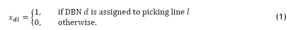
An approximation for the walking distance wlis defined as the size of the maximal SKU for picking line Í, while Vmaxis the largest volume of stock on a picking line over all picking lines. To make provision for carton utilisation, define the set of variables

and
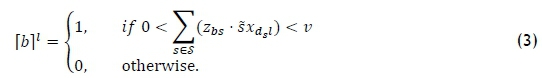
The variable [b]1 is set to 1 if the volume of store b's package from picking line l is less than a certain volume v, and 0 if the store's package from picking line l exceeds volume 𝑣, or if the store does not have a package from that picking line. The logical statement set (3) is written as if-then constraints in constraint sets (13)-(18). The out-of-DC date is taken into account by denoting the parameter dcurto be the current penalty associated with DBN d, the parameter doutto be the preferred number of days before DBN d's out-of-DC date that DBN d should be assigned to a picking line at the latest, and the parameter dtodto be the number of days until DBN d's out-of-DC date from the current day. The parameter dcuris initially set to 0 in the dynamic model, which indicates that if DBN d were to be assigned on the day it was released to the DC, it would be assigned on time. Define the variable
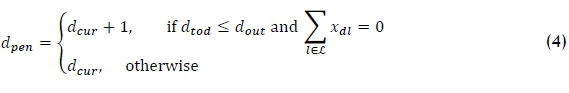
to be the penalty associated with DBN d for the following day for not being assigned to a picking line before a preferred date. This logical statement set is written as sets of if-then constraints in constraint sets (19)-(21).
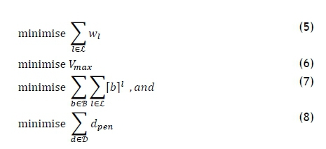
The objectives are therefore to
subject to
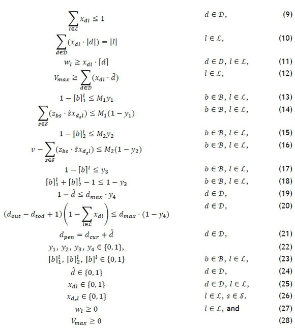
where M1= EsES(z6s ■ s) for b E S, M2= max{v, 1}, dmaj. = max{dou£ - d£od+ 1,1} for dED, and d is an auxiliary variable used in the sets of if-then constraints in constraint sets (19)-(21).
Objective function (5) minimises the walking distance of the pickers - i.e., the sum of the maximal SKUs over all picking lines. The second objective function (6) minimises the largest volume of stock on a picking line over all picking lines to ensure that stock is evenly distributed among the available picking lines. Objective function (7) minimises the number of packages whose volume is less than a specified volume, while the last objective function (8) minimises the total penalty incurred for DBNs not being assigned to a picking line before their preferred date.
Constraint set (9) ensures that each DBN is assigned to no more than one picking line. The fact that the number of locations that the assigned DBNs require must be equal to the number of available locations of a picking line is determined by constraint set (10), while constraint set (11) determines the size of the maximal SKU for each picking line. The largest volume of stock Vmaxon a picking line over all picking lines is determined by constraint set (12). Constraint sets (13)-(18) set [b]1to 1 if the volume of a certain store's package from a certain picking line is less than v, and to 0 if the store's package from that picking line exceeds volume v, or if the store does not have a package from that picking line. Constraint sets (19)-(21) penalise DBNs for being assigned to picking lines later than desired. The variable sets in (22)-(24) are used for the if-then constraint sets (13)-(21), while the variable sets (25)-(28) ensure that a DBN is either assigned to a picking line or not, a SKU is assigned to a picking line or not, the maximal SKU is non-negative, and the largest volume of stock on a picking line over all picking lines is non-negative.
Goal programming was used to assign a target to each objective function and weights to the deviational variables for each of these target values in order to determine a solution for the MOMKP. It takes approximately 15 minutes to find one Pareto optimal solution using the branch-and-bound technique in LINGO 11.0 [9] on a Macintosh OS X system equipped with a 2.6GHz Intel Core i5 processor and 8GB 1600MHz DDR3 SDRAM. This is not a reasonable amount of time. Ideally a set of solutions should be presented to the DM to decide which trade-offs need to be made. This results in a running time of two to three hours, which is excessive for the limited time that PEP's management has during the planning phase of the picking lines. Metaheuristics are thus developed in the following section to find a set of non-dominated solutions in a shorter time frame that are close to the Pareto frontier.
4 METAHEURISTIC APPROACHES
Quick algorithms need to be implemented, since three tiers must be addressed every morning during the planning phase of the picking lines, and a solution needs to be obtained from the PLAP before solving the SLP and OSP, shifting the focus more to the computational times of the algorithms to find a set of good solutions in less than a minute. Three metaheuristics are developed: the artificial bee colony algorithm, the genetic algorithm, and the memetic algorithm. These algorithms are chosen because they provide a set of good solutions upon termination instead of a single solution. The DMs can then decide which solution to implement, depending on their preference.
4.1 Artificial bee colony algorithm
The artificial bee colony (ABC) algorithm was first suggested by Karaboga [7]. The behaviour of honey bee swarms was the inspiration for the basic structure of the algorithm, due to the collective intelligence shared among the employed and unemployed foragers about their food sources. The ABC algorithm forms part of a group of swarm intelligence algorithms that have shown promising results in multi-objective optimisation problems, such as the multi-objective design optimisation of composite structures [14].
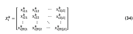
The foragers consist of employed bees, onlooker bees, and scout bees. The employed bees search and exploit food sources in the environment of recently-visited food sources in an attempt to find new regions containing flowers with a larger amount of nectar. They then travel back to the beehive to exchange information about their sources with the onlooker bees by means of a waggle dance in the dancing area, to communicate the location and profitability of their sources. Each onlooker bee decides which source to fly to, with each source having a certain probability that an onlooker bee will decide to pursue it. Sources containing more nectar will have a higher chance of having more onlooker bees exploiting their nectar. The profitability of a food source depends on its distance from the nest, the abundance of energy that it provides to onlooker bees, and the ease of extracting its nectar. If a food source is abandoned, scout bees discover new food sources by exploring the environment surrounding the beehive. A food source is represented by the solution, which is defined by the matrix

with
i the index of a food source - i.e., a feasible DBN assignment to picking lines,
|D| the number of DBNs initially in the storage racks that are considered to be assigned, and
|£| the number of available picking lines.
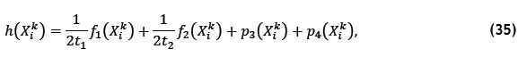
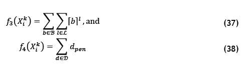
Each element xidlin the food source Xiis set to 1 if DBN d is assigned to picking line l, and to 0 if DBN d is not assigned to picking line l. An initial solution is determined by not violating any of the constraints in constraint sets (9)-(21). Penalty functions are used for objective functions (7) and (8) due to the DM wanting to have the percentage of small packages and the number DBNs that are assigned later than their out-of-DC date to be under a specified level. To use penalty functions while minimising objective functions (5) and (6) as much as possible, let
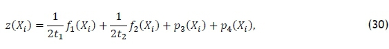
where
tj is the target value of objective function and
Pj(Xi) is the penalty function associated with function j in objective functions (7) and (8) for food source .
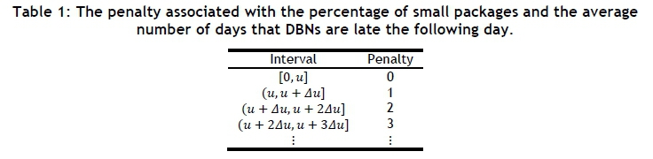
The functions
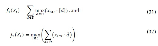
are defined exactly as in objective functions (5) and (6). Penalty functions p3(Xt) and p4(Xt) in equation (30) assign penalties linearly according to intervals for which a goal value u and an increment Δu need to be specified. The penalties are then assigned according to intervals, as seen in Table 1.
The nectar amount is given by the reciprocal 1/z(Xi). The probability of an onlooker bee selecting a certain food source k is given by
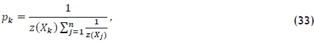
where η is the total number of food sources. Once an onlooker bee has found a food source2, it will extract nectar and find a neighbouring food source. This action is simulated in the algorithm by two actions. A random DBN from a random picking line is swapped with a DBN from another picking line in that solution with a specified probability a. If a DBN does not fit in the other DBN's picking line, it is sent to the storage racks, and one or more other random DBNs from the storage racks will be inserted into the available location(s) of that picking line to ensure that all \ l\ locations of the picking line are occupied by a SKU. In the second action a random DBN from a random picking line is replaced by one or more DBNs from the storage racks with a specified probability β. The equation a + β = 1 must hold. The employed bee will travel to this new food source if it is an improvement on the existing one, and inform the onlooker bees in the dancing area about the newly-found food source.
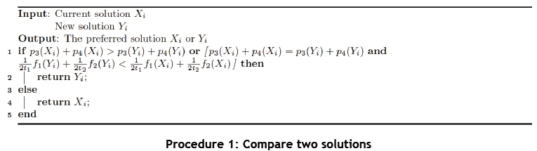
The new solution is then compared with the previous solution of the onlooker bee. Three cases may occur when comparing two solutions:
1. Any solution with no penalty is preferred to any solution with a non-zero penalty - i.e., a solution with p3(Xi) + p4(Xi) = 0 is preferred to a solution with p3(Xi) + p4(Xi) > 0.
2. When comparing two zero penalty solutions, the one having a smaller weighted objective function value is chosen - i.e., the solution having a smaller value for
.
3. When comparing two non-zero penalty solutions, the one having a smaller value for p3(Xi) + p4(Xi) is chosen. If the penalties are the same for both solutions, the solution having the smaller value for
is chosen.
A set of non-dominated solutions is maintained during the execution of the algorithm. An external archive is used to keep a historical record of all non-dominated solutions. During each iteration, feasible solutions are added to the external archive after which all solutions that are dominated by other solutions are removed from the external archive during the evaluation process. A solution, X1, with objective function values fj(X1) is said to dominate another solution, X2, with objective function values fj(X2) if (X1) < (X2) for each objective function j ε {1, ...,4}.
If an employed bee and onlooker bees cannot find an improving food source in a specified number of iterations, the employed bee's food source is abandoned. A scout bee then determines a randomly-generated food source, which is described as inserting DBNs from the storage racks into the available picking lines without violating constraints in constraint sets (9)-(21). The employed bee then travels to this food source, and the next iteration of the algorithm begins. The fact that scout bees generate random solutions ensures that diversity in solutions is maintained throughout the algorithm, which is vital to the success of multi-objective evolutionary algorithms. The algorithm terminates after a specified number of iterations. All feasible non-dominated solutions in the external archive are then returned to the decision-maker with their corresponding objective function values to determine which trade-offs need to be made.
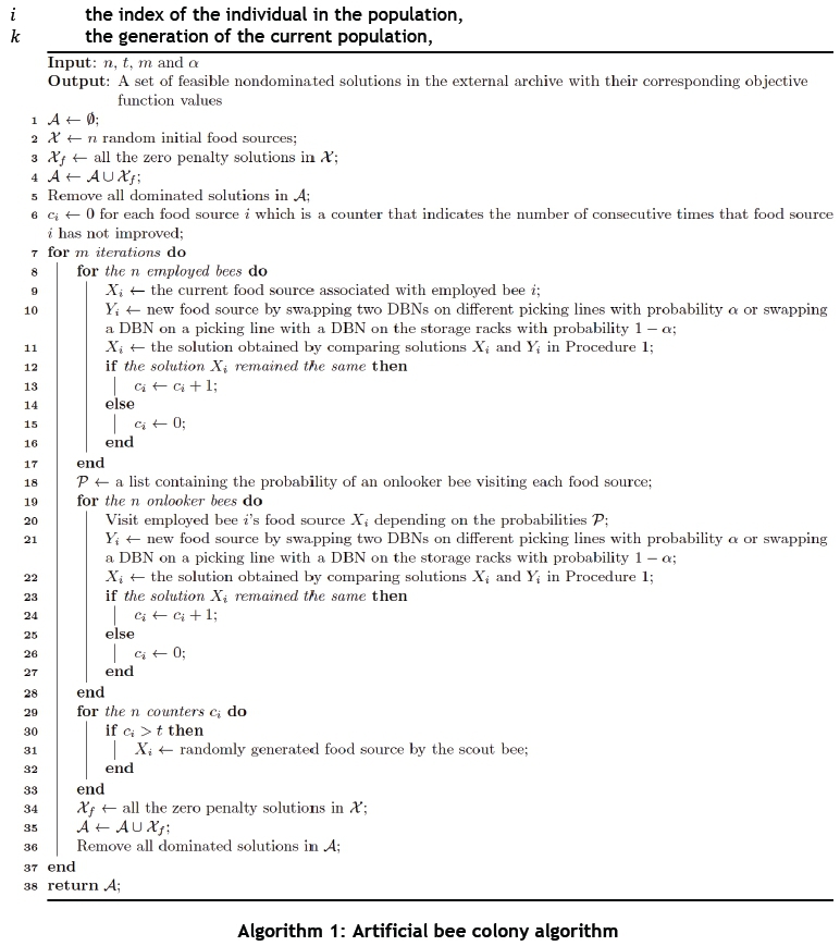
Algorithm 1 contains the pseudocode for the implementation of the ABC algorithm. It requires the number of food sources n, the number of unsuccessful trials t before a food source is abandoned by an employed bee, the number of times m that the bees search for food sources, and the probability a of swapping two DBNs from two different picking lines as input. The initialisation process takes place in lines 1-6, which represent the creation of the external archive A, generating η initial food sources X and setting counters ci to zero for each food source i that are used to determine when food sources are abandoned. The employed bees' phase follows in lines 8-17, while the onlooker bees' phase is given in lines 19-28. Lines 29-33 show that certain food sources are abandoned if better food sources are not found after t trials. The probability of an onlooker bee visiting each food source is determined between each employed bee's phase and each onlooker bee's phase, and the external archive is updated after each scout bee's phase in each of the m iterations. Procedure 1 contains the pseudocode to compare two solutions during the employed bees' phase and the onlooker bees' phase in lines 11 and 22 in Algorithm 1.
4.2 Genetic algorithm
The genetic algorithm (GA) was invented and proposed by John H. Holland in the early 1970s, and became popular after his book Adaptation in Natural and Artificial Systems [6] was published in 1975. The motivation that led to its creation came from Holland's interest in complex adaptive systems. All living organisms are made up of cells. A chromosome is made up of a collection of genes, with each gene defined as a block of deoxyribonucleic acid (DNA). Genes are used to form the characteristics of each individual3. The use of the GA to solve the PLAP was inspired by a study by Knowles and Corne [8] that focused on the implementation of a memetic algorithm for multi-objective optimisation.
A chromosome is represented by the solution (similar to that of the ABC algorithm), which is defined by the matrix
with
| D| the number of DBNs initially in the storage racks that are considered to be assigned, and | £| the number of available picking lines.
Each gene  in the chromosome is set to 1 if DBN d is assigned to picking line l, and to 0 if DBN d is not assigned to picking line l. The initial population is determined by inserting DBNs from the storage racks into a specified number of picking lines until all of the locations in all the picking lines contain a SKU for each individual4. This is analogous to the way the initial food sources are determined in Algorithm 1. All of the constraints in constraint sets (9)-(21) are always satisfied. The final similarity is that the fitness function is analogous to equation (30), which is given by
where  and
and  are defined exactly as in equations (31) and (32) by replacing xidl with
  . Tournament selection is used to select the individuals from the current population yfcand local archive 𝒜 𝑙;as parents to breed children for the offspring population 𝒫o. The local archive is synonymous with the external archive mentioned earlier in this section, which is initially empty. Binary tournament selection is used. It works by merging 𝒫 𝑘 and 𝒜 𝑙;into a single population
  , called the entire population. Groups of four individuals are randomly selected from
  ;in each of the n/2 iterations, where η is the size of the population. Each of these groups is independent of the others, meaning that an individual may feature in several of the groups. The first pair of individuals is evaluated, where the individual with the smallest value for
  is selected as a parent, after which the second pair is evaluated. The two selected parents in this group will then produce two offspring using the crossover operator. Working with groups of four rather than with pairs ensures that a parent does not breed with itself.
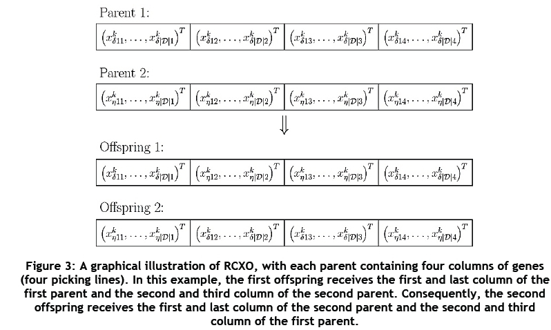
Two parents - say,  and
and  produce two children by using a crossover operator called the random column crossover operator (RCXO). RCXO selects a random parent for each of the |L| picking lines. For picking line λ, if parent
  was selected, then the first child will receive the genes from column
  and the second child will receive the genes from column
  . Similarly, if parent
  was selected, then the first child will receive the genes from column
  and the second child will receive the genes from column
  . An example of RCXO may be found in Figure 3 for the case when four picking lines are available.
RCXO may, however, cause individuals in yoto be produced that contain one or more DBNs that are assigned to two picking lines, which violates one or more constraints in constraint set (9). This problem is fixed by using a repair operator that removes a random duplicate DBN and places one or more DBNs from the storage racks in their place. This process is repeated until all assigned DBNs are assigned to only one picking line. Once the children have been repaired, each child is mutated according to a specified probability μ. Mutation is performed by removing a certain number of DBNs from the picking lines and replacing them with DBNs from the storage racks. This enables diversity in  , since previously unassigned DBNs from the storage racks are now allowed to be assigned to a picking line; and this potentially causes an individual to be more fit.
Once all children have been generated after performing the repair and mutation operators, only the children that represent zero penalty solutions are added to  . The local archive
  is then updated by removing all solutions that are dominated by another solution in
  . If the number of non-dominated solutions in
  is more than a specified maximum size of
  , solutions are removed according to the concept of the crowding distance [2] given by the formula
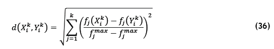
for solutions Xtkand Yf with  , and where
fjmaxis the maximum value for function j for all the solutions in  and
and
fjminis the minimum value for function j for all the solutions in  .
.
The functions
are equivalent to objective functions (7) and (8).
In this case,  and
and  are used in conjunction with
  and
and  to determine the distance between solutions in the four-dimensional objective function space. The local archive
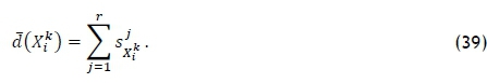
  grows too large in the experimental tests in section 5. The computational time saved by managing a smaller local archive can be used to increase the number of iterations that can be performed by the algorithm. As a result, a size restriction is imposed to avoid the algorithm from being computationally expensive. Let
 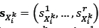 be the vector containing the distances
  of the r nearest neighbours of solution
  , with
  being the distance of the nearest neighbour,
  being the distance of the second nearest neighbour, and so on; then the total crowding distance of a solution
  may be given by
The  ; solutions with the smallest value for
  are then removed from
  where
where  is the size of
  ;before any solutions are removed. The best 50 per cent of the individuals - those with the lowest fitness value in equation (35), from
  - then proceed to the following generation to produce the next offspring population with
  .
.
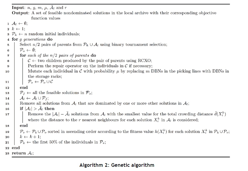
The pseudocode for the implementation of the GA may be found in Algorithm 2. It requires the population size n, the number of generations g until the algorithm is terminated, the number of DBNs m to be removed from the picking lines by replacing them with DBNs from the storage racks during mutation, the probability μ of mutating an individual's chromosome, the maximum size 𝑛 of the local archive, and the number of nearest neighbours r to be considered when removing individuals from the local archive as input to be executed. The initialisation process takes place in lines 1-3, which represent the initiation of the local archive  ;and generate η initial individuals in Pk. The offspring population 𝒫𝑜 is produced in lines 5-12, where the crossover, repairing and mutation take place. All feasible solutions in 𝒫𝑜 are added to
  ;after which all non-dominated solutions in ;are kept, as is evident in lines 13-15. If the size of
  ;is greater than a specified limit, then solutions are removed from
  ;according to the total crowding distance in equation (39), which may be seen in lines 16-18. Finally, the current population for the following generation is determined in lines 19-21.
The GA is then extended to a memetic algorithm (MA), which applies a local neighbourhood hill-climbing (LNH) algorithm to a child with a specified probability after the crossovers, repairing, and mutation have taken place in the genetic part of the algorithm. In each iteration of the LNH algorithm, a new solution is determined either by swapping two DBNs assigned to different picking lines in the best found solution, or by swapping a DBN assigned to a picking line with one or more DBNs on the storage racks in the best found solution. The best found solution is then updated to the new solution if the new solution's fitness value is
better than the best found solution's fitness value. This process is repeated for a specified number of iterations. The LNH algorithm was chosen to play a role in solving the MOMKP, since other local searches are too computationally expensive for the problem, or have the potential to lead the search away from promising regions in the domain that the GA managed to explore. The MA requires additional computation than does the GA, due to the local search.
5 RESULTS
Historical data [11] was collected by PEP over a period of 12 weeks, of which seven weeks were used for static and dynamic testing. Historical solutions are currently found by hand by the picking line managers. In the static testing, the DBNs released for the present day, and the DBNs that are in the storage racks in the historical case, were used to determine whether the ABC algorithm, GA, and MA could assign a subset of these DBNs to the picking lines in a better way than was the historical case for that specific day. The DBNs that are available for that day for the algorithm to use in this testing are dependent on the DBNs assigned on the previous days in the historical case, and not on the DBNs that the respective algorithm assigned on the previous days. Dynamic testing is carried out by starting with the same set of DBNs as the historical case on the first day of assignment. The assigned DBNs in the preferred solution produced by the respective algorithm for the current day are then removed from the set of available DBNs, and the DBNs released on the following day are then added to the set of available DBNs. The algorithm uses this new set of DBNs to assign DBNs for the following day. The DBNs that are available for a specific day for the algorithm are thus independent of the DBNs assigned on the previous days in the historical case, but instead are dependent on the DBNs assigned by the specific algorithm on the previous days.
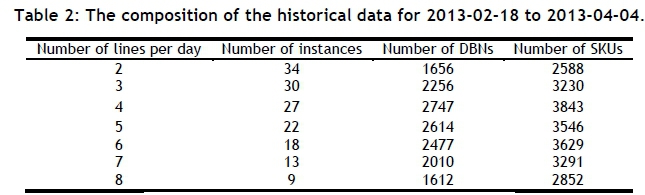
The original data set contained 61 working days, where each day had a specific number of available picking lines for that day, ranging from two to 11 picking lines [12]. The data set was converted into seven data sets, where each set has a constant number of scheduled picking lines for each day of picking, ranging from two to eight picking lines. This allows for an accurate comparison between the historical case and the algorithms. The re-organisation was achieved by removing picking lines from each historical day of picking while preserving the DBNs that were picked on that day - i.e., the DBNs in the new dataset are a subset of the DBNs in the original dataset. Table 2 summarises the modified historical data for the seven-week period used in the static and dynamic testing.
All tests were executed on a Macintosh OS X system equipped with a 2.6GHz Intel Core i5 processor and 8GB 1600MHz DDR3 SDRAM. The mathematical formulations were coded and solved in LINGO 11.0, after which it was concluded that it was impossible to solve a real-world problem and present a set of solutions in a reasonable amount of time. All algorithms presented were implemented in Python 3.3 [16].
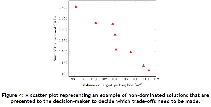
Parameter calibration was performed for each of the algorithms to determine which combination of parameter settings provides the best results in the allocated time. It was decided that the parameters η = 15, m = 50, t = 4 and a = 0.5 be used for the ABC algorithm, and η = 15, g = 50, m = 5 and μ = 0.5 be used for the GA and MA. For the MA, five iterations were performed each time LNH was executed; the probability of performing LNH on an individual was taken as 0.2; and the probability of swapping two DBNs from two different picking lines was chosen to be 0.25. Once an algorithm has terminated, the DM is presented with a set of non-dominated solutions to decide which trade-offs need to be made in terms of the walking distance (the sum of the maximal SKUs) and the maximal volume of stock (the largest volume of stock on a picking line over all picking lines). Figure 4 contains a scatter plot of  , showing an example of a set of non-dominated solutions. It is evident from this plot that, when moving from one solution to another, one of the objective functions increases while the other one decreases.
5.1 Static testing
The first two objective function values - the sum of the maximal SKUs (the walking distance of the pickers) and the maximal volume of stock - are compared for all the algorithms and the historical case. The DBNs released for the present day and the DBNs that are in the storage racks in the historical case were used to determine whether the ABC algorithm, GA, and MA could assign a subset of these DBNs to the picking lines in a better way than the historical case for that specific day. The DBNs that are available for that day for the algorithm to use in this testing are dependent on the DBNs assigned on the previous days in the historical case, and not on the DBNs that the respective algorithm assigned on the previous days. The algorithm thus solves, for each day, the same problem that was solved historically. This explains the static nature of the results performed in this section.
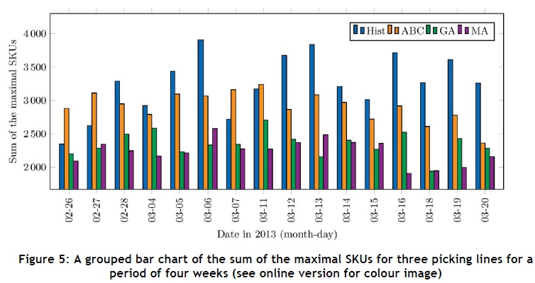
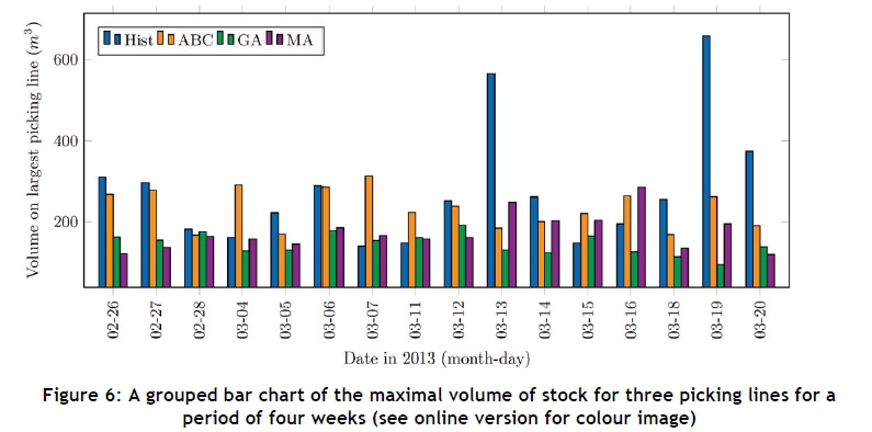
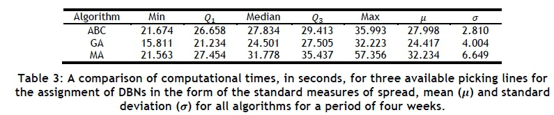
Figures 5 and 6 contain the results for the first two objective functions by means of grouped bar charts for a period of four weeks for three picking lines. The values in both figures for a specific day correspond to the same solution. Out of the 16 days of picking in the four-week period, 12 days show an improvement for the first objective and 11 days show an improvement for the second objective for the ABC algorithm. There is an on-average 5.12 per cent decrease in the first objective and a 1.98 per cent increase in the second objective. For the GA, there is an improvement 16 days of the time for the first objective, and an improvement 13 days of the time for the second objective. The average decrease is 23.64 per cent and 34.97 per cent for the first and second objectives respectively. Lastly, there is an improvement in 16 of the days for the first objective and 12 of the days for the second objective for the MA, with an average decrease of 25.70 per cent and 23.05 per cent for the first and second objectives respectively. A comparison of computational times for three available picking lines is shown in Table 3 for all the algorithms.
5.2 Dynamic testing
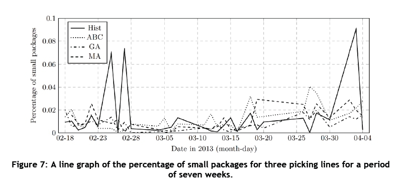
To compare the percentage of small packages and the average days that late DBNs are assigned later than their out-of-DC date to the historical case, the ABC algorithm, GA, and MA need to assign the DBNs in a dynamic sense. This is carried out by starting with the same set of DBNs as the historical case on the first day (2013-02-18 in the testing performed in this section) of assignment. The assigned DBNs in the preferred solution produced by the respective algorithm for the current day are then removed from the set of DBNs, and the DBNs released on the following day are added to the set of DBNs. The algorithm uses this new set of DBNs to assign DBNs for the following day. The DBNs that are available for a specific day for the algorithm are independent of the DBNs assigned on the previous days in the historical case, but instead are dependent on the DBNs assigned by the algorithm on the previous days.
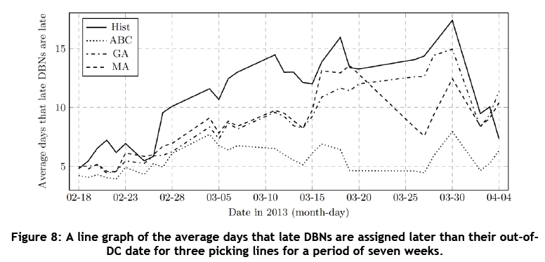
Figures 7 and 8 display the results for the percentage of small packages and the average days that late DBNs are assigned later than their out-of-DC date, respectively, in the form of line graphs for a period of seven weeks for three picking lines. It is clear that all of the algorithms were able to maintain the percentage of small packages, avoiding the rapid increases in the percentage of small packages compared with the historical case. The GA shows the lowest percentage of small packages over the seven-week period. The average days that late DBNs are assigned later than their out-of-DC date show a decrease of 20 per cent when using the GA, and 22.08 per cent when using the MA, compared with the historical data. The ABC algorithm performs the best in terms of assigning DBNs no later than their out-of-DC date, with an average decrease of 48.97 per cent in the average days that late DBNs are assigned later than their out-of-DC date.
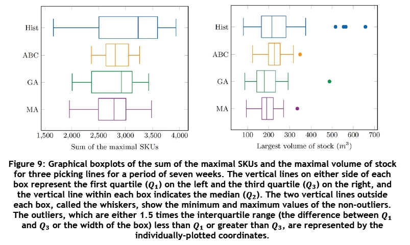
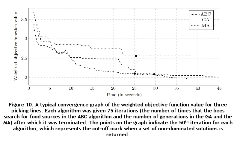
The graphical boxplots in Figure 9 indicate that the sum of the maximal SKUs and the maximal volume of stock shows an improvement in the dynamic testing for all of the tested algorithms. Convergence graphs for the tested algorithms may be found in Figure 10. The values on the y-axis are the weighted objective function values given by the formula
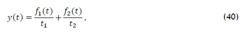
where ft( t) is the objective function value for objective i at time t and ttis the target value for objective . The points on the plot represent the cut-off mark of 50 iterations for each algorithm. The ABC algorithm flattens out prematurely, while the GA and MA continue to decline. The weighted objective function value for the MA does not improve significantly after the GA's cut-off mark. In this regard it is suggested to use the GA instead of the MA.
6 CONCLUSION
An order picking system in a distribution centre (DC) owned by Pep Stores Ltd (PEP), consisting of parallel unidirectional picking lines, was investigated. Order picking is a labour-intensive task, and the cost associated with order picking accounts for approximately 55 per cent of all operating costs in a DC. SKUs that differ only in size classification are grouped together in a single DBN, and must be picked in the same wave. Previous studies suggested that improvements needed to be made when determining which DBNs to assign to which picking lines on a given day, and when to leave DBNs for the following day [13].
The problem was formulated as a multi-objective multiple knapsack problem where the picking lines may be viewed as the knapsacks and the DBNs as the items to be inserted into the knapsacks. The artificial bee colony algorithm, the genetic algorithm and the memetic algorithm were implemented to approximate the Pareto frontier for the first two objectives while using penalty functions for the last two objectives. Penalty functions allow the percentage of small packages and the average number of days that DBNs are assigned later than their out-of-DC date to be kept under specified limits while minimising the first two objectives.
It is recommended that PEP use the genetic algorithm to assign DBNs to the available picking lines, since it performed best in both the static and the dynamic cases. The genetic algorithm showed an average decrease of 23.64 per cent and 34.97 per cent in the walking distance of the pickers and the largest volume of stock on a picking line over all picking lines respectively. The percentage of small packages was maintained, with a 20 per cent decrease in the average number of days that DBNs are assigned later than their out-of-DC date.
Future work may include the implementation of other nature-inspired algorithms, such as the artificial immune system and particle swarm optimisation algorithms, to see the effect they have on the provided solutions, compared with the algorithms developed in this study. Scheduling techniques could be applied to determine on which day a specific DBN should be assigned to a picking line. This is different from the dynamic case, where DBNs are only to be considered for assigning on the present day. All of the algorithms presented in this study, and other nature-inspired algorithms, could be tested when a single DBN could be picked from multiple picking lines by splitting DBNs into smaller DBNs. Lastly, different picking line configurations found at PEP's DCs could be analysed using the implemented algorithms.
REFERENCES
[1] De Villiers, A.P. 2011. Minimising the total travel distance to pick orders on a unidirectional picking line, Master's Thesis, Stellenbosch University, Stellenbosch. [ Links ]
[2] Deb, K., Pratap, A., Agarwal, S. & Meyarivan, T. 2002. A fast and elitist multiobjective genetic algorithm: NSGA-II, IEEE Transactions on Evolutionary Computation, 6(2), pp 182-197. [ Links ]
[3] Fidanova, S. 2007. Ant colony optimization and multiple knapsack problem, pp 498-509 in Rennard, J.P. (Ed.), Handbook of Research on Nature Inspired Computing for Economics and Management, London: Idea Group Reference. [ Links ]
[4] Fivaz, D. 2013. SKU duplication on a unidirectional picking line, Master's Thesis, Stellenbosch University, Stellenbosch. [ Links ]
[5] Gandibleux, X. & Freville, A. 2000. Tabu search based procedure for solving 0-1 multiobjective knapsack problem: The two objective case, Journal of Heuristics, 6(3), pp 361-383. [ Links ]
[6] Holland, J.H. 1975. Adaptation in natural and artificial systems, University of Michigan Press. [ Links ]
[7] Karaboga, D. 2005. An idea based on honey bee swarm for numerical optimization, Erciyes University, Turkey (unpublished). [ Links ]
[8] Knowles, J.D. & Corne, D.W. 2000. M-PAES: A memetic algorithm for multiobjective optimization, Proceedings of the 2000 Congress on Evolutionary Computation, 1(1), pp 325-332. [ Links ]
[9] LINDO Systems. 2015. Lingo 11.0. Available from www.lindo.com. [ Links ]
[10] Matthews, J. 2015. SKU assignment in a multiple picking line order picking system, PhD Thesis, Stellenbosch University, Stellenbosch. [ Links ]
[11] Matthews, J. & Visagie, S.E. 2014. Picking line problems. Available from scholar.sun.ac.za/handle/10019.1/86110. [ Links ]
[12] Matthews, J. & Visagie, S.E. 2014. Order sequencing on a unidirectional picking line, European Journal of Operational Research, 231(1), pp 79-87. [ Links ]
[13] Matthews, J. & Visagie, S.E. 2015. SKU assignment using correlations on unidirectional picking lines, ORiON, 31(2), pp 61-76. [ Links ]
[14] Omkar, S., Senthilnath, J., Khandelwal, R., Narayana Naik, G. & Gopalakrishnan, S. 2011. Artificial bee colony (ABC) for multi-objective design optimization of composite structures, Applied Soft Computing Journal, 11(1), pp 489-499. [ Links ]
[15] Pep Stores Ltd. 2015. PEP. Available from www.pepstores.com. [ Links ]
[16] Python Software Foundation. 2015. Python 3.3. Available from www.python.org. [ Links ]
[17] Wei, X. & Zhang, K. 2012. Discrete artificial bee colony algorithm for multiple knapsack problems, International Journal of Advancements in Computing Technology, 4(21), pp 484-490. [ Links ]
Submitted by authors 25 Aug 2016
Accepted for publication 27 Feb 2017
Available online 26 May 2017
* Corresponding author svisagie@sun.ac.za
# The author was enrolled for an MCom (Operations Research) degree in the Department of Logistics, University of Stellenbosch
1 A wave is defined by three actions: (1) placing DBNs in their locations on the picking line, (2) picking orders, and (3) clearing out possible leftover stock from the locations after the picking has been completed.
2 A food source contains only one employed bee, but may contain more than one onlooker bee.
3 The word 'individual' refers to the chromosome, fitness value, and all characteristics associated with the individual, whereas 'chromosome' refers to the gene structure of the individual.
4 The size of the population must be an even number to keep the population constant, since two children are produced by two parents.

