FEATURE ARTICLES

 

Probability management and the flaw-of-averages^#

 

 

P.S. Kruger; V.S.S. Yadavalli

Department of Industrial and System Engineering, University of Pretoria, South Africa

 

 

---

ABSTRACT

Uncertainty is ever-present and is an integral part of life. Recognising the existence of uncertainty and its possible effects on decision-making may be important for the profitability, financial success, or even survival of an organisation. A relatively new discipline, - known as probability management, - has recently emerged as part of operations research/management science. This paper will attempt to provide a brief introduction to the concepts of probability management and the motivation behind its development. One of the major driving forces resulting in this development is the phenomenon known as the 'flaw-of-averages'. The flaw-of-averages has important consequences in industrial engineering, financial, business, and economic models. The classic newsvendor problem will be used as an illustrative example. However, the main purpose of this paper is to discuss the most important characteristics of the flaw-of-averages. It will investigate and attempt to quantify some of the generic factors that may have an influence on the existence and severity of the flaw-of-averages and its expected consequences. Various models will be developed, and experiments will be conducted using Microsoft Excel as a modelling tool and an experimental approach based on Monte Carlo simulation modelling.

---

OPSOMMING

Onsekerheid is altyd teenwoordig, en is 'n integrale deel van die lewe. Die herkenning van die bestaan van onsekerheid en die moontlike gevolge vir besluitneming mag belangrik wees vir die winsgewendheid, finansiële sukses en selfs die voortbestaan van 'n organisasie. 'n Relatief nuwe konsep het onlangs verskyn as deel van operasionele navorsing / bestuurswetenskap bekend as waarskynlik-heidsbestuur. Hierdie artikel sal poog om 'n kort inleiding te verskaf tot die konsep van waarskynlikheidsbestuur en die motivering agter die ontwikkeling daarvan. Een van die belangrike dryfvere agter hierdie ontwkkeling is die fenomeen bekend as die 'gemors-vangemiddeldes'. Die gemors-van-gemiddeldes het belangrike gevolge in bedryfsingenieurswese, finansiële, ekonomiese en besigheids-modelle. Die klassieke koerantverkoperprobleem sal as n illustratiewe voorbeeld gebruik word. Die hoofdoelwit van hierdie publikasie is egter om die mees belangrike eienskappe van die gemors-van-gemiddeldes te bespreek. Dit sal sommige van die belangrikste generiese faktore wat 'n invloed mag hê op die bestaan en die erns van die gemors-van-gemiddeldes ondersoek, en poog om die verwagte gevolge daarvan te kwantifiseer. Verskeie modelle sal ontwikkel word, en eksperimente sal uitgevoer word deur gebruik te maak van Microsoft Excel en 'n eksperimentele benadering gebaseer op Monte Carlo simulasie modellering.

---

 

 

1 INTRODUCTION

Statistical thinking will one day be as necessary for efficient citizenship as the ability to read and write. H G Wells (1866-1946)

The world is "living on the edge of uncertainty" [1]. Any planning exercise is involved with the future. Crossing the boundary between the known present and the uncertain future represents a jump into the mysterious unknown. Organisations spend large amounts of money on planning exercises that inevitably include expensive efforts - for example, insurance - to mitigate the possible negative effects of the uncertain future. If not enough is known about a subject there is a tendency to classify it as random, and therefore as unfathomable and uncontrollable. However, science is continually attempting to push the envelope of knowledge and the barriers of the unknown, and thus move into the realm of what may be considered as unknown, or at least as uncertain.

1.1 Historical perspective

In mediaeval times, the throw of a die was controlled by the gods until Girolamo Cardano (1501 -1579) proved otherwise [2]. Uncertainty is everywhere in one form or another. This is not new, and has been a part of the human condition since time immemorial. The Roman scholar, Pliny the Elder (23-79), declared: "In these matters the only certainty is that nothing is certain"; and Benjamin Franklin (1706-1790) maintained that: "Nothing is certain except death and taxes". Furthermore, it seems as if the level of uncertainty is increasing, given the existing and ever-increasing political, social, and economic turmoil in the world. One may choose to ignore the existence of uncertainty or assume that nothing can be done about it. However, the consequences of uncertainty in the business of everyday life may be quite severe. Fortunately, Blaise Pascal (1623-1662) and Pierre de Fermat (1601-1665) laid the foundations of probability theory some time ago, and people such as Abraham de Moivre (1667-1754), Sir Francis Galton (1822-1911), and Sir Ronald Aylmer Fisher (18901962), among many others, developed statistical models and descriptive statistics [2]. These developments and their enhancements over the years provide the tools at least to analyse uncertainty, investigate its origins and possible effects, and maybe even to quantify it to some extent.

1.2 New developments

Apart from the ongoing development of the theory of mathematical statistics, some other more recent developments facilitate the effective application of mathematical statistics. The availability of inexpensive and powerful computer hardware and software greatly increases the ability to handle the extensive computational load often required. Furthermore, the traditional complaint of the statistician about not having enough data is disappearing, and quite the contrary may be true, since "we are drowning in a sea of data and data insecurity" [3]. Data bases in use today, containing zeta bytes of raw data, are not uncommon. These developments, techniques, and models are certainly not perfect. The results of, and conclusions based on, the application of a statistical technique, possibly based on huge amounts of data, to investigate and analyse uncertainty are, of necessity, mostly subject to their own form of uncertainty - such as those embedded in statistical inference. But these uncertainties are, at least to some extent, controllable and quantifiable. Even so, the application of mathematical statistics in a structured and consistent way to real-world problems has become mandatory. It may provide at least some insight into and understanding of the structures of the stochastic processes surrounding us, and may especially enable the evaluation of the severity of the possible consequences of uncertainty and how to plan and be prepared for it in advance. This paper intends to illuminate some of these concepts.

 

2 BACKGROUND

This section is intended to provide some background information that may be required for the rest of this paper. A reader with intimate knowledge of Monte Carlo simulation, spreadsheet software, Jensen's inequality, or the flaw-of-averages may skip this paragraph without loss of continuity.

2.1 Monte Carlo simulation

Anyone who attempts to generate random numbers by deterministic means is, of course, living in a state of sin. John von Neumann (1903-1957)

Simulation modelling has gone through some remarkable developments over the last 50 or 60 years, and has become one of the most widely-used techniques available to industrial engineers and managers for modelling and designing complex stochastic systems [4]. Techniques such as system dynamics, discrete/continuous simulation, agent-based approaches, and the plethora of associated software products, are commonplace. However, the Monte Carlo method is the basis of any kind of simulation model intended to model and investigate stochastic processes.

Regarding Figure 3, a random number, R, from a distribution, in this case normal, may be generated. By substituting this value into the input/output transformation function of the model, F(X), the output value, Y, may be obtained. The essence of the Monte Carlo method consists of repeating this process several times [5].

 

 

 

 

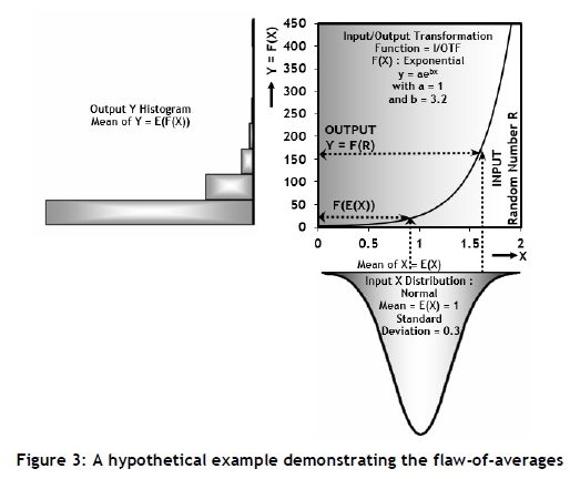
This process is a typical, albeit very simplified, example of what is known as a Monte Carlo simulation model. The Monte Carlo method was first formulated by John von Neumann (1903-1975) and Stanislaw Ulam (1909-1984) as part of their research for the Manhattan Project [2]. Monte Carlo simulation seems, at present, to be the only viable way to investigate the existence and extent of what is known as the flaw-of-averages (see sections 2.3 and 2.4), and will be used extensively for this purpose in this paper. Furthermore, Monte Carlo simulation is used quite extensively in industrial engineering, management and financial analysis (especially for risk analysis), and project scheduling [6,7,8,9]. Monte Carlo simulation will be used extensively as a modelling approach in this paper.

2.2 Spreadsheet software

Despite their drawbacks, spreadsheets have overwhelmingly become the analytical vernacular of management. Sam L Savage

Spreadsheets certainly have some severe drawbacks, especially as a general purpose platform for model development; but they also have some significant advantages [5]. They are widely available, and probably have the largest and most diversified user base of any single software product. Spreadsheet software is known, used, and trusted by almost every engineer, business manager, and accountant. Almost everyone has become accustomed to the rapid, interactive responses available from spreadsheet applications, even though they are slow in terms of execution speed. This may present a problem in the case of large Monte Carlo simulations requiring large sample sizes and using only standard spreadsheet software. Applicable commercial software, usually available as spreadsheet add-ins that address this problem to some extent, are available from companies such as Palisade Corporation and Frontline Systems Inc., and new developments may be expected [10, 11, 12]. Spreadsheet software, specifically Microsoft Excel, will be used exclusively in this paper for the model development and execution.

2.3 Jensen's inequality

The worst form of inequality is to make unequal things equal. Aristotle (384-322 BC)

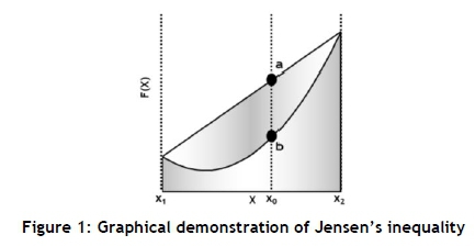
The mathematical basis of the so-called flaw-of-averages (FoA) [13] may be found in a mathematical concept known as Jensen's inequality [14]. It is named after the Danish mathematician Johan Jensen (1859-1925) who defined and proved it in 1906, and relates the value of a convex function of an integral to the integral of a convex function. In its simplest form, the inequality states that the convex transformation of a mean is less than or equal to the mean after convex transformation; it is a simple corollary that the opposite is true for concave transformations. Jensen's inequality may be demonstrated as shown in Figure 1.

With reference to Figure 1, for an arbitrarily chosen value of X = xo, if a is a point on the secant line of the function between x1 and x2, and b is a point on the graph of the function. It is clear that:

a > b for all values xi < X < X2

In the context of probability theory, Jensen's inequality is generally stated in the following form: If X is a random variable with expected value E(X), and F(X) is a convex function, then

F(E(X)) < E(F(X))

where F(E(X)) is the function of the expected value and E(F(X)) is the expected value of the function.

This is often known as the flaw-of-averages (FoA) [13] and may be stated as:

The function of the expected value (mean) is less than or equal to the expected value (mean)of the function.

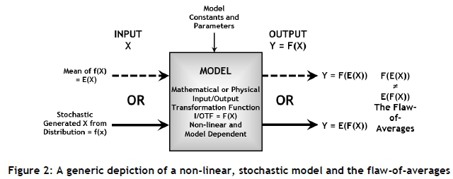
2.4 The flaw-of-averages

The law-of-averages. This often misused, so-called 'law' is a layman's term without any valid mathematical basis. It is also known as the gambler's fallacy [15].

The variance of a stochastic variable has traditionally been used, and still is used, as a measure of variation and uncertainty. The dictum 'a mean without a standard deviation does not mean much' is still true, but the standard deviation may not provide the complete picture. The so-called flaw-of-averages may be present in numerous industrial engineering and business models - for example, quality control, inventory management, reliability engineering, financial planning, budgeting, project management, maintenance planning, investment analysis, marketing, risk analysis, and most simulation models - to name but a few [5,7,8,9]. The FoA may also be stated as "average inputs do not always result in average outputs" [16]. Often, planning for the future or making predictions dependent on uncertain inputs and outcomes is replaced by a single, constant, so-called average number [17,18]. This leads to a class of systematic errors that is called the flaw-of-averages [5]. All that is required for the existence of the FoA is for the model to have a non-linear input-output transformation function, and for at least one of the model input variables to be subjected to uncertainty. The FoA may be illustrated as shown in Figure 2. The FoA and the Monte Carlo method may be further demonstrated by using the hypothetical example shown in Figure 3. The summary results for this example, as shown in Table 1, were obtained by designing and executing a Monte Carlo model with a sample size of 10 replications, each consisting of 1,000 observations. The results shown in Table 1 indicate that F(E(X)) < E(F(X)), as predicted by Jensen's inequality, and the existence and severity of the flaw-of-averages is obvious, as indicated by the flaw-of-averages percentage defined as FoA% = [E(F(X)) - F(E(X))] / F(E(X)). The discussion and investigation of the FoA is the main focus of this paper.

 

3 PROBABILITY MANAGEMENT

Nearly all organisations worship at the false altar of determinism. Steve Roemerman, as quoted by Kirmse and Savage [19]

A relatively new discipline, known as probability management, has recently emerged as part of operations research/management science [11,12,19,20,21]. The principles of probability management are by no means new or unknown, but have recently come under the spotlight and, in conjunction with risk analysis and other kinds of financial analysis, are one of the major applications of spreadsheet software and Monte Carlo simulation. Actuaries have been using the principles of probability theory and statistical analysis for many years, and industrial engineering techniques -such as quality control and reliability engineering - are well-established. Advances in computer technology are well-known. It may be these advances and the availability and popularity of spreadsheet software that have highlighted the problems associated with the FoA. Ironically, however, these same advances and developments may be instrumental in resolving these problems.

"Probability management could be a new paradigm that shifts traditional decision-making from the reliance on point estimates (i.e., the mean-variance paradigm), to decision-making that addresses the variability and more complex relationships affecting decision-making environments" [22]. "The main focus of probability management is on estimating, maintaining, and communicating the distribution of the random events driving a business" [20]. The principles and structure of probability management were defined in two seminal papers by Savage, Scholtes, and Zweidler that were published in OR/MS Today in 2006. They not only initiated this new discipline and defined some initial structures, but gave it a name and therefore a much-needed identity. Probability management seems to be a natural progression and development from relative deterministic information systems to decision-making supported by stochastic-systems thinking.

Probability management, as defined so far, rests on three main concepts [22]:

Interactive simulation of complex stochastic and non-linear systems provides engineers and managers with enhanced decision support and, perhaps more importantly, with timely and a better understanding of, and insight into, the multi-faceted characteristics and uncertainty of their environment.

Stochastic libraries involve the gathering, maintaining, and disseminating of all data of a stochastic nature that may be of importance to the organisation. The data should be analysed and manipulated into suitable formats for example, statistical distributions and other primary statistical models and should be made available for decision-making over different computing platforms. These libraries and sub-models collectively may be an important asset for any organisation, similar to other assets - such as people, equipment, and facilities - and should be treated as such.

A certification authority, which may be a separate department in an organisation and that will be responsible for the management of all probability management activities. These may include the gathering and dissemination of the appropriate data, the specification of the required data structures, and the development and dissemination of modelling expertise.

The FoA (see section 2.4) is one of the primary driving forces behind the development of probability management, and is the main topic of the rest of this paper.

 

4 THE NEWSVENDOR PROBLEM

What you lose on the swings you gain on the roundabouts! Attributed to P G Wodehouse (1881-1975)

It seems that most applications of the flaw-of-averages have been concerned with applications of financial analysis, although some other applications have been reported [22,23]. However, a large number of instances in industrial engineering and general management may also exist [5,7,9]. As a typical generic example, consider the newsvendor model, a well-known, classical inventory theory model [24]. What is now known as the newsvendor problem - first mentioned in 1888 by Francis Isidro Edgeworth (1845-1926) [25] - is arguably the beginning of stochastic inventory control theory. The simplest variant of the newsvendor problem may be formulated as follows [24]:

A company buys and sells a single product every day.

C_o is the unit cost of overage.

C_u is the unit cost of underage.

The demand per day is a continuous non-negative random variable.

The statistical distribution function of the demand is f(x) and the cumulative distribution function is F(x).

The decision variable is the order quantity Q, the number of units to buy at the beginning of a day.

The objective is to determine the value of the order quantity Qopt that will minimise the expected total overage and underage cost at the end of the planning period.

Figure 4 shows the input/output transformation function (I/OTF) of the newsvendor problem for different values of the cost ratio Cu/Co. The I/OTF is piecewise linear and discontinuous, and should therefore be classified as non-linear (see section 5.3) except for Cu/Co = 1. Furthermore, at least one input, the demand, is subjected to uncertainty, and the I/OTF is convex. Thus a FoA should be expected, and the flaw-of-averages percentage (FoA%) should be negative.

Assume the following values for the input parameters:

C_o = 50, C_u = 100 and the demand has a normal distribution with a mean of 3,000 units and a standard deviation of 1,000 units. The optimum order quantity, Qopt, may be determined from the following formula [24]:

Qopt = F^-1[(C_u /(C_u+C_o))] = 3,431 units

where F^-1(x) is the inverse distribution function of the demand.

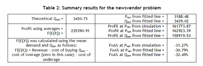
The newsvendor problem has numerous applications. It is used, for example, by airlines to determine so-called 'optimum over-booking' [25,26]. Given these assumptions, it may minimise the expected total overage and underage cost. However, it may not maximise the expected profit and, furthermore, disregarding the flaw-of-averages may cause a significant over-estimation of the expected profit, as shown in Table 2.

A Monte Carlo simulation model for the newsvendor problem was designed and executed with a sample size of 100 replications, each consisting of 1,000 observations. The results are summarised in Table 2.

This formulation of, and solution to, the newsvendor problem suffers from some limitations. For example, the sales and purchase prices are not included, and thus Qopt is the value of the order quantity that minimises the sum of the overage and underage (O/U) cost but does not necessarily provide the value of the order quantity that will maximise the profit, Popt. Furthermore, though the distribution of the demand is taken into account, the possible FoA is ignored.

The problem may be enhanced slightly by including the following input parameters and output quantities:

C : Sales price per unit = 100,

P : Purchase price per unit = 200,

V : Salvage value per unit not sold = 90,

P_opt : The order quantity that will maximise the profit, and

FoA% : The flaw-of-averages percentage defined as [E(F(X))-F(E(X))]/FE(F(X)).

With these additional variables, a Monte Carlo simulation model may be constructed, providing the summary results shown in Table 2 and Figures 5, 6, and 7. Furthermore, Popt was obtained by running the simulation model for a specific value for the order quantity, and with a sample size of 1,000 observations (days), replicated 100 times.

 

 

 

 

 

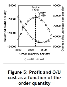
From Table 2 and Figures 5 and 6 it seems as if:

The theoretical value for Qopt (3430.73) and the value obtained from the simulation (3409.02) is almost equal, validating the simulation model to some extent (see Table 2).

According to the simulation, the maximum profit occurs at Popt and not at Qopt (see Figure 5).

The flaw-of-averages is obviously present and significant (see Table 2).

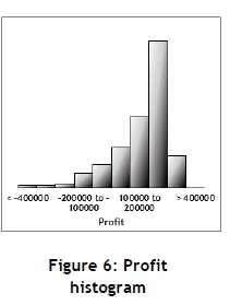
The Monte Carlo simulation may also provide some other useful information. For example, Figure 6 shows the profit distribution (histogram), which is not symmetrical even though the input has a normal distribution and thus is symmetrical. Furthermore, Figure 7 shows the risk profile from which estimates of the upside/downside risk [5] for any value of an assumed profit may be obtained. For example, an estimate of the probability of making a loss (approximately 0.14) may be determined from the risk profile.

 

5 MONTE CARLO SIMULATION EXPERIMENTS

If your experiment needs statistics, you ought to have done a better experiment. Ernest Rutherford (1871-1937)

The factors influencing the existence and severity of the flaw-of-averages (FoA) may be classified as those factors that are inherently present in most problems (generic), or factors that are problem-dependent. The purpose of Section 5 is mainly to investigate, and maybe quantify, the influence of some generic factors using an experimental approach based on Monte Carlo simulation modelling. The influence of the following generic factors on the FoA will be considered:

The severity of the non-linearity of the input/output transformation function (see Sections 5.2 and 5.3).

The type of input distribution (normal, beta, etc.) (see Section 5.4).

The standard deviation of the input distribution (see Section 5.5).

The mean of the input distribution (see Section 5.6).

The coefficient of skewness of the input distribution (see Section 5.7).

Multiple stochastic input variables (see Section 5.8).

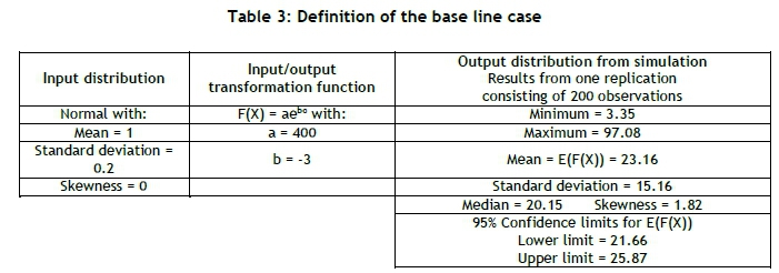
5.1 The base line case

A base line case will be used for reference and comparison purposes; its characteristics and parameter values are defined in Table 3. The base line case was designed to be as simple as possible, but still contain the basic components of a Monte Carlo simulation model intended to investigate the FoA. All the other experiments in Section 5 will be executed with the same experimental approach, sample size, characteristics, and parameter values as those used for the base line case, unless otherwise stipulated for the purpose of the specific experiment.

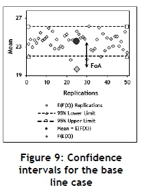
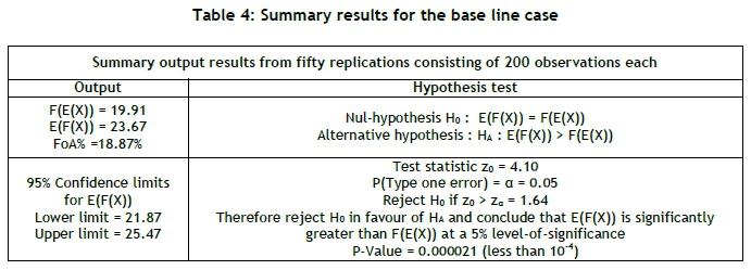
The base line case is used to obtain an idea of the stochastic stability and the required sample size. Figures 8 and 9 indicate that a simulation run of 200 observations should be adequate from the viewpoints of both stochastic stability and confidence intervals. All the experiments in Section 5 will be conducted with a simulation run length of 200 observations, replicated 50 times, resulting in a total sample size of 10,000 observations. The summary results for the base line case are shown in Table 4. The use of a replication approach is often required to provide independent observations for valid statistical analysis. This may not be necessary in this specific case, but will nevertheless be followed.

 

 

 

 

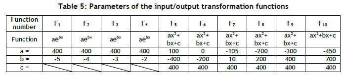
5.2 The non-linearity of the input/output transformation function

The existence of non-linearity in the input/output transformation function (I/OTF) is a key requirement for the existence of the flaw-of-averages. Several I/OTFs with different non-linearities were chosen, as shown in Figure 10, with parameter values defined in Table 5.

 

 

It is necessary to be able to quantify the severity of the non-linearity of a specific function. For the purposes of this paper, a coefficient of non-linearity (CONL) was defined, regarding Figure 1, as follows:

CONL = (Area below the linear function - Area below the non-linear function) / (Area below the linear function).

Defined in this way, the value of the CONL will be between -1 and +1, with negative values indicating concavity, positive values convexity, and a value of zero indicating linearity.

Figure 11 illustrates the effect of the value of the CONL on E(F(X)) and FoA%, and Figure 12 shows the FoA% and CONL for the various functions.

 

 

 

 

5.3 Discontinuous input/output transformation functions

A discontinuous input/output transformation function is often found as part of industrial engineering and business models. It usually results from factors such as quantity discounts, tax breaks, moving from one technology to another, or as an inherent characteristic of the model logic such as that encountered in the newsvendor problem (see Figure 4). Furthermore, using computer programming nomenclature, whenever an IF-statement appears as part of the formulation of the model logic, it may cause a discontinuity and thus a flaw-of-averages (FoA), although all the functions may be piecewise linear. Figure 13 shows three arbitrarily-chosen, discontinuous, but piece-wise linear functions, and Table 6 provides the results. The FoA, even in this case, is obvious.

 

 

5.4 Different types of distributions

Numerous well-known statistical distribution models are available to be used as input models to a stochastic model [27]. One of the difficult decisions that is part of any simulation modelling effort is the identification of the appropriate statistical distribution to be used for a specific stochastic input variable. If sufficient and applicable data is available, several statistical procedures [28] may be employed to make a motivated decision. Alternatively, possible knowledge of the underlying characteristics of the stochastic process under consideration may be contemplated. In Section 5, the triangular distribution will be used extensively, since it is an appropriate and convenient choice for purposes of experimentation for the following reasons:

Firstly, the triangular distribution is flexible since it has three parameters the minimum, a, the mode, c, and the maximum, b. The triangular distribution is often used in simulation modelling when very little or no historical data is available, and because it may provide a reasonably good fit for many other distributions [4]. Estimating values of the parameters of, for example, a skewed gamma distribution when no data is available may prove difficult. However, estimates for the values of the parameters of a triangular distribution may often readily be obtained from some knowledge of the characteristics of the stochastic process of interest [4].

Secondly, since the triangular distribution has three parameters, it is possible to obtain values for these parameters by predefining required values for the mean, standard deviation, and coefficient of skewness. This neccessitates the solving of a set of non-linear simultaneous equations, which was achieved in this case by using the generalised revised gradient (GRG) optimisation algorithm that is part of the solver add-in available in MicroSoft Excel.

Six distributions were chosen for the experiments in Section 5.4: The normal (base line case), beta, logistic, rectangular, triangular, and Laplace distributions. These are all symmetrical distributions, well-known and widely-used. The gamma and exponential distributions were not included since they are inherently skewed, and could influence the results (see Section 5.7). The chosen input distributions are shown in Figures 14 and 15. Table 7 shows the chosen constant values of the parameters, and Figures 16, 17, and 18 summarise the results obtained from the Monte Carlo simulation experiments.

 

 

 

 

 

 

 

 

 

 

Figures 16 and 17 seem to indicate that significant differences might exist between the various distributions. Furthermore, the Laplace distribution seems to be an outlier, as supported by the information provided by Figure 18. The reason that the Laplace distribution is different may be found in its excessive peakedness (Figure 15), a kurtosis excess value of 3 (Table 7), and the fact that it is leptokurtic together with the beta and logistic distributions. To prove a possible difference between the various distributions, a standard analysis of variance (ANOVA) test [28] was performed, the results of which are summarised in Table 8. These results indicate that there is a significant difference between the various distributions. However, this test does not identify which distributions are causing the difference. This may be resolved by employing a multiple comparison test, such as the Fisher least significant difference (LSD) test [28]. The results of the Fisher LSD test are summarised in Figure 19.

Regarding Figure 19, there seems to be a significant difference (five percent level of significance) in the influence on the FoA between:

The normal, triangular, logistic, and Laplace distributions;

The logistic, rectangular, and Laplace distributions;

The beta and Laplace distributions; and

The rectangular and Laplace distributions.

Although some of these differences are small (see Figures 16 and 17), the choice of the type of input distribution should be done with care and circumspection.

5.5 Different standard deviations

The different triangular input distributions used in this experiment are shown in Figure 20 and the parameter values defined in Table 9. The results are summarised in Figure 21. It seems that the standard deviation does have a significant influence on the FoA.

 

 

 

 

5.6 Different means

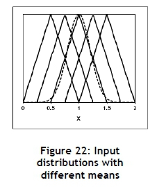
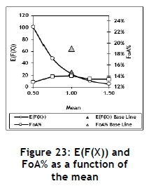
The different triangular input distributions used in this experiment are shown in Figure 22 and the parameter values defined in Table 10. The results are summarised in Figure 23. It seems that the mean does have a significant influence on the FoA, as measured by E(F(X)) but not by FoA%. This is probably due to the fact that the FoA% is also a function of the mean.

 

 

 

 

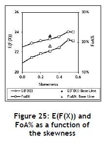
5.7 Different skewness

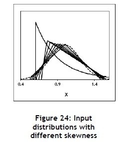
The different triangular input distributions used in this experiment are shown in Figure 24 and the parameter values defined in Table 11. The results are summarised in Figure 25. It seems that the skewness does have a significant influence on the FoA. Since the value of the coefficient of skewness for the triangular distribution is limited to a maximum of approximately 0.56, the exponential distribution with a coefficient of skewness of 2 was included. This resulted in an E(F(X) of 34.74 and an FoA% of 29.23%, further stressing the influence of the skewness on the FoA. The exponential distribution has only one parameter, the mean, which is equal to the standard deviation. It is therefore not very flexible, and it is impossible to define the mean and standard deviation independently. However, by introducing an off-set, as shown in Figure 24, it was possible to obtain the parameter values shown in Table 11, which are approximately equal to those required.

 

 

 

 

5.8 Multiple input

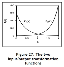
Most stochastic models have two or more input variables subjected to uncertainty. If the output associated with each input is further transformed by an additional transformation, such as multiplication, it may amplify the FoA even further. Figure 26 displays two different input distributions, and Table 12 defines the distribution and input/output transformation function parameter values. Figure 27 shows the associated input/output transformation functions, and Table 13 summarises the results. The simple secondary transformation of multiplying the two values to obtain the output amplifies the FoA severely.

 

 

 

 

 

 

6 CONCLUSIONS AND CAVEATS

This is not the end, it is not even the beginning of the end, but it is maybe the end of the beginning. Winston Leonard Spencer Churchill (1874-1965)

The adage 'On average we should be OK', will be not OK on average! The all-too-common practice of blissfully disregarding uncertainty by substituting average values into a stochastic model with a non-linear input/output transformation function may result in a significant flaw-of-averages. As illustrated in this paper using a simple base line case and subsequent experiments, whenever the input/output transformation function of a model is in some way nonlinear, and at least one of the input variables is subjected to uncertainty, the flaw-of-averages will be present and may be severe.

It was demonstrated that all the generic factors investigated may influence the extent to which the flaw-of-averages exists significantly. Ignoring the possible presence of the flaw-of-averages may result in dire future consequences for any organisation. The tools and techniques to investigate and manage the flaw-of-averages are available and should be applied, albeit with circumspection.

Probability management and its future developments may provide a mind-shift for engineers and managers to move away from the paradigm of determinism and averages to the much-needed proper consideration of the characteristics and consequences of uncertainty. This may provide companies with improved decision-making and therefore higher profits. New techniques and approaches are continuously being developed at a rapid rate.

The results and conclusions of Section 5 provide some insight into the characteristics of the flaw-of-averages that may be of some value. However, these results should only be seen as guidelines, and only valid within the experimental frame defined by the assumed maximum and minimum values of the respective parameter and variable values.

The Monte Carlo simulation approach may have some inherent disadvantages; and the same is true for spreadsheet software as a modelling platform [5]. Nevertheless, the Monte Carlo approach, using Microsoft Excel and possibly some appropriate and available add-ins, seems at present to be the most viable and accessible way of investigating the existence and extent of the flaw-of-averages with relative efficiency and ease.

This paper employed a theoretical and experimental approach, without any practical examples. However, further research is being conducted that will investigate and discuss the possible influence of the flaw-of-averages on the calculation of compound interest and net present value.

To teach how to live with uncertainty, yet without being paralysed by hesitation, is perhaps the chief thing that philosophy can do. Bertrand Arthur William Russell (1872-1970).

 

REFERENCES

[1] Brooks, M. 2015. On the edge of uncertainty. Profile Books Ltd.         [ Links ]

[2] Bernstein, P. L. 1996. Against the Gods: The remarkable story of risk. John Wiley & Sons.         [ Links ]

[3] Peterson, A. 2014. We are drowning in a sea of data. Washington Post, 20 February, 2014.         [ Links ]

[4] Kelton, W. D. Sadowski, R. & Sadowski, D. A. 2002. Simulation with Arena. McGraw-Hill.         [ Links ]

[5] Savage, S. L. 2003. Decision making with insight. Thomson Brooks Cole.         [ Links ]

[6] Apostolakis, G. E. 2007. Engineering risk benefit analysis, available from ocw.mit.edu, last accessed on 20 May 2016.         [ Links ]

[7] Barlow, J. F. 1999. Excel models for business and operations management. John Wiley & Sons.         [ Links ]

[8] Winston, W. L. 2000. Decision making under uncertainty with RISKOptimizer. Palisade Corporation.         [ Links ]

[9] Winston, W. L. 2001. Simulation modelling using @RISK. Duxbury Thomson Learning.         [ Links ]

[10] Savage, S. L. & Thibault, J. M. 2015. Towards simulation networks or the medium is the Monte Carlo. Proceedings of the 2015 Winter Simulation Conference, USA.         [ Links ]

[11] Saigal, S. 2009. Probability management in action, available from www.analytics-magazine.org, last accessed on 20 May 2016.         [ Links ]

[12] Sweitzer, D. 2012. Simulation in Excel: Tricks, trials and trends, available from sites.google.com, last accessed on 20 May 2016.         [ Links ]

[13] Savage, S. L. 2002. The flaw of averages, Harvard Business Review, November, 2002.         [ Links ]

[14] Weisstein, E. W. 2016. Jensen's inequality, available from mathworld.wolfram.com, last accessed on 24 May 2016.         [ Links ]

[15] Rees, N. 1966. Cassel dictionary of word and phrase origins. Cassel & Co.         [ Links ]

[16] Savage, S. L. 2009. The flaw of averages: Why we underestimate risk in the face of uncertainty. John Wiley & Sons.         [ Links ]

[17] Domanski, B. 2000. Averages, schmaverages! Why you should not use averages for performance prediction. available from www.responsivesystems.com, last accessed on 20 May 2016.         [ Links ]

[18] Parish, S. 2012. The flaw-of-averages. Entrepreneurs, October, 2013.         [ Links ]

[19] Kirmse, N. & Savage, S. L. 2014. Probability management 2.0. OR/MS Today, (5).         [ Links ]

[20] Savage, S. L. Scholtes, S. Zweidler, D. 2006 a. Probability management. OR/MS Today, (1).         [ Links ]

[21] Savage, S. L. Scholtes, S. & Zweidler, D. 2006 b. Probability management, Part 2, OR/MS Today, (2).         [ Links ]

[22] Méndez Mediavilla, F. A. & Hsun-Ming, L. 2011. Using data marts for probability management in supply chains, available from swdsi.org/swdsi2011/, last accessed on 20 May 2016.         [ Links ]

[23] Li, W. Zhang, F. & Jiang, M. 2008. A simulation- and optimisation-based decision support system for an uncertain supply chain in a dairy firm. Int. J. Business Information Systems, (2).         [ Links ]

[24] Winston, W. L. 1994. Operations research, applications and algorithms. 3^rd edition, Duxbury press.         [ Links ]

[25] Hill, A. V. 2016. The newsvendor problem, Clamshell Beach Press.         [ Links ]

[26] Pak, K. & Piersma, N. 2002. Airline revenue management: An overview of OR techniques, 1982-2001, ERIM Report Series, Research in Management, available from core.ac.uk, last accessed on 26 may 2016.         [ Links ]

[27] Evans, M. Hastings, N. & Peacock, B. 2000. Probability distributions, John Wiley & Sons.         [ Links ]

[28] Montgomery, D. C. & Runger, C. R. 2011. Applied statistics and probability for engineers, John Wiley & Sons.         [ Links ]

 

 

Submitted by authors 24 Jun 2016
Accepted for publication 10 Aug 2016
Available online 6 Dec 2016

 

 

# This paper is dedicated to the memory of our mentor, Professor Kris Adendorff, who introduced us, some years ago, to the abyss that may exist between the deterministic and the stochastic worlds.
* Corresponding author:paul.kruger12@outlook.com