GENERAL ARTICLES

 

Solving the dial-a-ride problem using agent-based simulation

 

 

I. Campbell^*; M.M. Ali; M.L. Fienberg^#

School of Mechanical Industrial & Aeronautical Engineering, University of the Witwatersrand, South Africa

 

 

---

ABSTRACT

The 'dial-a-ride problem' (DARP) requires a set of customers to be transported by a limited fleet of vehicles between unique origins and destinations under several service constraints, including within defined time windows. The problem is considered NP-hard, and has typically been solved using metaheuristic methods. An agent-based simulation (ABS) model was developed, where each vehicle bids to service customers based on a weighted objective function that considers the cost to service the customer and the time quality of the service that would be achieved. The approach applied a preprocessing technique to reduce the search space, given the service time window constraints. Tests of the model showed significantly better customer transit and waiting times than the benchmark datasets. The ABS was able to obtain solutions for much larger problem sizes than the benchmark solutions, with this work being the first known application of ABS to the DARP.

---

OPSOMMING

Die 'bel-'n-rit' probleem' (DARP) vereis dat kliënte, met 'n beperkte vloot van voertuie tot die diensverskaffer se beskikking, tussen unieke oorspronge en bestemmings onder verskeie diens beperkings vervoer word. Die probleem word beskou as NP-hard, en word gewoonlik opgelos met behulp van meta-heuristiese metodes. 'n Agentgebaseerde simulasie (ABS) model is ontwikkel, waar elke voertuig mik om kliënte te bedien, gebaseer op 'n geweegde doelfunksie wat die koste vir die kliënt en die tyd gehalte van die dienslewering in ag neem. Die benadering pas 'n voorafverwerking tegniek toe om die soek spasie, onderhewig aan die diens tyd venster beperkings, te verminder. Simulasie resultate toon noemenswaardige verbeteringe wanneer die kliëntediens transito- en wagtye as maatstaf gebruik word. Die ABS kon oplossings kry vir veel groter probleemgroottes as die maatstaf oplossings. Hierdie werk is die eerste bekende toepassing van ABS om die 'bel-'n-rit' probleem aan te spreek.

---

 

 

1 INTRODUCTION

The door-to-door transportation of people or goods forms part of an extensively-studied set of vehicle-routing problems (VRPs) involving the use of combinatorial optimisation, a sub-field of operations research. Most vehicle-scheduling and -routing problems are a variation of the capacitated vehicle-routing problem (CVRP), which generalises the well-known 'travelling salesman problem' (TSP). The CVRP with time windows for deliveries is called the 'capacitated vehicle-routing problem with time windows' (CVRPTW).

A variation of the CVRPTW is the vehicle-routing problem with pick-up and deliveries (VRPPD), which allows for mixed servicing of customer requests for the delivery of goods. Vehicle routes are determined to service specific customer collection and drop-off requests, while considering the customers' goods load sizes and the pick-up vehicles' load capacity. Each transport request is between a single origin and destination, with no transhipment of goods taking place. The same vehicle has to perform both the pick-up and the delivery of customer goods. The dial-a-ride problem (DARP) is an extension of the VRPPD, where the loads to be transported are represented by people and is considered as one of the most complex VRPs [1]. Problems can either be for a single or multi-vehicle scenario, and possibly with different vehicle capacities.

Specifically, the DARP occurs when customers phone to request a transport service, where the customers are typically elderly, sick, or disabled. Like a VRP, the DARP services n number of customers with a fleet of m vehicles. However, DARP requires vehicle routes and schedules that accommodate requests from customers who have specified where they must be collected from, where they must be dropped off, and times when it is convenient for them to be picked up and dropped off. This makes the DARP a many-to-many type of VRP, where each customer has their own starting and ending route nodes. In some cases, customers may require a return trip between their travel points later in the day [2]. All vehicles start and end at a common depot, with customers typically sharing rides.

The DARP is characterised by conflicting objectives. It must minimise transportation costs, like the VRP, while also having to consider minimising user time inconvenience. It should also maximise the number of customers serviced per vehicle. For a DARP, requests are typically collected and vehicle routes scheduled by a central planning unit that must determine how to allocate customers to vehicles. The problem is more complicated than just partitioning customers into clusters, as consideration of the time sequence in which customer requests occur must be accounted for. The DARP is considered to be NP-hard; thus one cannot expect to find a global optimal solution in polynomial time. Rather, a robust algorithm that is able to provide a good solution should be used [3].

 

2 LITERATURE REVIEW

2.1 DARP

The aim in solving a DARP is to obtain the optimal fleet size and capacity configuration to satisfy all customer requests [2]. A solution should satisfy the following conditions:

• All pick-up and delivery requests are fulfilled;

• Transhipments of goods or people may not occur on the route;

• The load of a vehicle cannot exceed its capacity; and

• An objective is to minimise a cost function [4].

The DARP includes time-constrained intervals in which the servicing of customers should take place. Thus the objective function of a DARP usually considers a user inconvenience factor to measure the quality of the service offered. This makes the DARP harder to solve than typical transportation problems, as a weighted objective function between cost and time is needed. In the event that strict time windows are used, transportation costs are high. Similarly, having low-cost vehicle routes can result in customers having long travelling and waiting times. Therefore a balance between service quality and routing costs must be sought [5]. Typically there will be an upper bound on the maximum customer transportation time constraint [2].

The presence of time window constraints makes the solution space of a CVRPTW highly non-convex, making it easy to move from a feasible to a non-feasible solution space. Solution methods may be designed for strict service time windows (called 'hard' time windows) or for 'soft' time windows. Soft time windows allow for a degree of violation to balance customer service and cost requirements, while hard time windows do not [6]. Solution methods may be designed for hard or soft time windows. For example, for the DARP, Cordeau and Laporte [7] use soft time windows to achieve low route costs, whereas Cubillos et al. [8] use hard time windows to achieve good customer service.

When solving a static DARP, three decisions are required. These are (1) determining how to cluster the customers to be serviced by the same vehicle, (2) sequencing the servicing of customers into a vehicle route within their assigned cluster, and (3)scheduling the customer pick-up and drop-off events for each vehicle [7]. Two common solution methods are used. One is by making use of insertion heuristics, whereby customers are optimally inserted into an initial route, making the solution quality reliant on the sequence in which customers are visited. The second is to use cluster-first and route-second heuristics. This approach partitions all the customers into a number of subsets, equivalent to the number of vehicles available to service the customers. Optimal routes are then determined for each specific vehicle to service its customer subset. The quality of the solution obtained relies on the effectiveness of the partitioning [9].

2.2 Mathematical formulation of the DARP

The DARP has been modelled mathematically in numerous works, with each work proposing slight variations in formulation. Typically, a DARP consists of n customer requests, where each customer specifies a pick-up location i and drop-off location n+i. Customers indicate a preferred earliest pickup time a_iand drop-off time bn+i. There is a fleet of \K| vehicles of constant capacity Q_k that start at an origin depot and end at a destination depot.

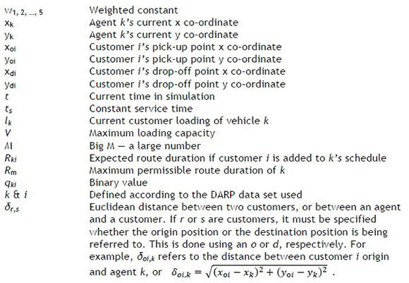
An example of a mathematical formulation is given by Cordeau [11]. The following variables and constant sets are defined over a directed graph:

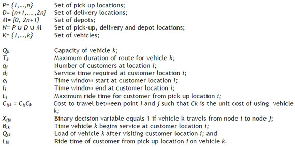
The DARP can be defined mathematically as:

Subject to:

 

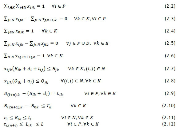
The objective function (2.1) can be a simple distance minimisation function [10], or a multi-criteria objective function [11], minimising the total transportation costs and customer transportation time inconvenience. The cost elements used commonly relate to the fixed vehicle costs for each kilometre travelled, and the cost-per-minute for servicing customers linked to the driver's wages [3]. Service quality can be determined by making a comparison between the direct and excess ride times a customer spends travelling to his destination, and the time spent waiting before departure [2].

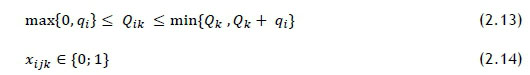
Constraints (2.2) and (2.3) ensure that each customer is only serviced by a single vehicle and that the delivery of a customer takes place on the same route as the customer pick-up. Constraints (2.4)-(2.6) ensure that each vehicle route starts and ends at the origin and destination depots respectively. Flow conservation of time and load at the nodes is ensured by constraints (2.7) and (2.8). The ride times are defined by (2.10) and limited by (2.12). The latter also acts as precedence constraints. The duration of routes is limited by (2.10), and (2.11) and 2.13) are time window and capacity constraints respectively.

2.3 Solution techniques

The DARP is an NP-hard combinatorial problem; therefore few exact algorithms exist to solve it, and they are only able to solve small problem sizes. Heuristic and metaheuristic methods have been widely applied to solve larger DARPs, and have enabled solutions to be obtained for increasingly large and complex problems (see [12]).

The type of algorithm that can be used to solve a DARP depends on the number of customers. Typical techniques used to solve DARP include custom heuristics and metaheuristic methods based on tabu search (TS), simulated annealing (SA), and genetic algorithms (GA). Classical heuristics for VRPs can be classified into the categories of route construction methods, two-phased methods, and route improvement methods. These methods include a population mechanism, which uses elements of the current solution for the next solution. A new approach of classical heuristic methods is the inclusion of learning mechanisms to improve on current solutions or to restart solving the problem with a different set of rules or parameters [13].

The Clark and Wright savings algorithm is one of the most widely-known routing heuristics. It aims to make route cost savings by combining customers into the same route, rather than servicing them separately, to reduce the total vehicle distance travelled. The cost savings are defined by S_ij = c_i0 +c_0j-c_ij, where i is a customer on one route, and j another customer on a second route. Routes are merged together if S_ijis positive, with the heuristic able to operate both in parallel or sequentially. The algorithm is time-consuming to implement, as distances, costs and savings need to be calculated between all customers [14].

Cordeau and Laporte's TS algorithm [7] constructs an initial solution by randomly assigning customer requests to vehicles, with an infeasible solution permissible. Their algorithm follows a typical TS method, considering and implementing neighbourhood moves. Each route move is measured against the objective function, which aims to minimise route duration and ride times. One type of move is defined as removing a customer request from a route and inserting it into another route. Another move type is an intra-route interchange. The algorithm was applied to data sets varying in size, the largest being 144 customer requests with 13 vehicles.

Zidi et al. [10] proposed an approach that uses a multi-objective simulated annealing algorithm that minimises both cost and a service quality condition. Service quality (SQ) was defined as a function of both customer ride time (RT) and the number of customer stations visited (NSV), where SQ = RT+NSV (2.24). The algorithm used the two-phased approach of cluster-first, route-second. The initial route constructing was done by a random assignment of vehicles to the transportation requests. They also apply a neighbourhood improvement search in the second phase of the algorithm to improve their solution.

A genetic algorithm approach was used by Cubillos et al. [8], where time windows were considered as hard constraints. When Zidi et al. [10] considered soft time windows, their vehicle ride times were largely similar to those obtained by Cubillos et al. [8], and significantly outperformed Cordeau and Laporte's (2003) customer ride times [7].

Both Jorgensen et al. [15] and Cubillos et al. [8] apply their own version of a genetic algorithm to the same dataset of the DARP, using a cluster-first route-second approach. In both cases a genetic algorithm is used for the clustering, with Cubillos et al. [8] using a preprocessing step before commencing with the clustering. This involved constructing a preliminary precedence table to reduce the search space of feasible solutions. The table considers each time event associated with a customer pick-up or delivery, and whether other events have to occur before or after the specific event. An incompatible list of customers that can be serviced by the same vehicle can be determined. Pre-processing of time events allows the genetic algorithm to search a smaller solution space, with less chance of moving into infeasible solution spaces [8].

Cordeau and Laporte's [7] tabu search algorithm was able to yield better vehicle route durations, but did not provide better customer ride time durations than the methods used by Cubillos et al. [8] and Jorgensen et al. [15].

2.4 Agent-based simulation

Agent-based simulation has been gaining increasing importance as a method to use in simulating complex systems, but with limited coherence in the literature on how an ABS should be applied. An ABS is generally characterised by [16]:

• Agents operating in an environment that is beyond their control.

• A simulated environment that forms part of the model by providing the required infrastructure. The simulated environment may perform auxiliary tasks or assist with the interaction between agents.

• A step-wise execution approach where all agent actions occur sequentially, with no event occurring in between the discrete event steps.

Events in an ABS are the set of all possible actions that may occur (e.g., customer pick-up or dropoff). Depending on the definition of the ABS, events may be either dependent or independent of time and may occur concurrently to one another, or may trigger another action. Entities in ABSs can play either an active role (being considered an agent) or a passive role (being considered an object). An agent is differentiated from an object in that:

• It has a physical dimension that forms its body, and is able to sense and interpret its environment.

• It is capable of performing multiple actions that consume a specific amount of time to be performed. Actions can be triggered by a sensor, with the outcome of an action deemed to be either a success or failure.

• An agent is closely interlinked with action processes. One action may activate other agent actions that form a process, with the possibility of actions occurring concurrently. A process would continue to run until it reaches a successful outcome or it is terminated due to a failure [16].

The use of ABS for solving VRPs is limited in the literature, with applications focusing on the general CVRP. Zeddini et al. [17] solve a dynamic VRP using a multi-agent system consisting of vehicle, bidder, and client agents. The authors used an objective function to minimise the number of vehicles used and the distance travelled. Vokrinek et al. [18] use a multi-agent approach for a VRP that must minimise route costs and the number of vehicles used. Their model solved the VRP in polynomial time. This approach did not outperform the benchmark results, but it did yield relatively good solutions in short computing times.

Barbucha and Jedrzejowicz [19] propose a two-agent parallel model to solve a VRP that must service up to 199 customers. Their algorithm was unable to yield better results than a tabu search method applied to the same data set.

ABS is not well known outside the narrow ABS community, with limited application of the method beyond the purposes of scientific, educational, and experimental use. ABS is still considered to be in the early stages of development, with no widely-accepted and proven methodology existing for the development of an ABS. The complexity required to construct an ABS is considered vast, given that it is not based on traditional mathematical computational methods. The computational requirements of an ABS can be intensive as the number of agents increases. This is due to the design of an ABS, which usually imposes communication requirements between agents that are not scaled linearly [20]. This is also evident from applications in the literature, where the number of customer requests modelled does not exceed 200.

 

3 METHODOLOGY

3.1 DARP Instances

DARP instances, consisting of 20 test scenarios, were developed by Cordeau and Laporte [7]. These are based on realistic assumptions, and include time windows, vehicle capacities, route durations, and maximum ride durations obtained from real data from the Montreal Transit Commission. The test scenarios are diversified by the number of vehicles available, and range between 24 and 144 customer requests, with some of the different test scenarios summarised in Table 1. Each scenario has a unique depot location defined as the average location between all customer node points. (Refer to Cordeau et al. [21] for a detailed description of this procedure.) All scenarios had half the data sets with customers specifying collection time windows, and the other half of the customers specifying delivery time windows. The time of day was from 0 to 1440 minutes (24 hours). Travel time is equal to the Euclidean distance between the nodes. The input data files for the test scenarios are accessible at http://neumann.hec.ca/chairedistributique/data/darp/tabu/.

 

 

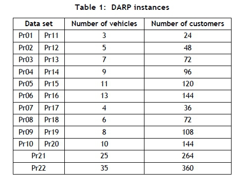
The ABS model was tested using two additional data sets, labelled Pr21 and Pr22. These data sets were created to establish whether the proposed approach was able to yield feasible solutions for larger numbers of agents and customers. The location of the depots for these data sets was set to the average of the x and y co-ordinates of all customer nodes. Data set Pr21 was composed from Pr02, Pr04, and Pr05, and data set Pr22 was composed from Pr01, Pr02, Pr03, Pr04, and Pr05.

All the data sets in Table 1, except for Pr21 and Pr22, have benchmark solutions provided by Cordeau and Laporte [7] that were obtained using a tabu search algorithm.

3.2 Evaluation of ABS model performance

The performance metrics determined for each of the test scenarios were:

• The total cost (distance travelled) to service all customer requests;

• The total customer waiting time incurred for customers to be picked up from their origin;

• The total customer transit time.

The results obtained from the ABS were compared with the benchmark results obtained by Cordeau and Laporte [7]. Customer waiting and service times were also compared with results from Jorgensen et al. [15] and Cubillos et al. [8].

Cordeau and Laporte [7] provide results detailing the total cost, total customer waiting time, and total customer transit times. Jorgensen et al. [15] and Cubillos et al. [8] only provide the total customer transit times in their solutions. Solutions common to all authors exist for data sets Pr01, Pr02, Pr03, Pr05, Pr11, Pr12, P13, Pr15, Pr17, and Pr19. Some solutions sets provided by Cordeau and Laporte [7] are incomplete, only providing the total cost to service all customers (Pr04, Pr07, Pr08, Pr13, Pr14).

Strictly speaking, since Cubillos et al. [8] and the ABS model in this work use hard time windows, and Cordeau and Laporte [7] use soft time windows, the cost results are not comparable. However, a smaller difference in cost will still give an indication of better solution quality.

Computer processing time taken to solve the instances was noted. All programming and solving was done using MATLAB R2007b on a Lenovo laptop computer with Intel i5 core processor, CPU 2.3 GHz, 4.00 GB RAM, and Windows 8.1 Professional operating system.

3.3 ABS model description

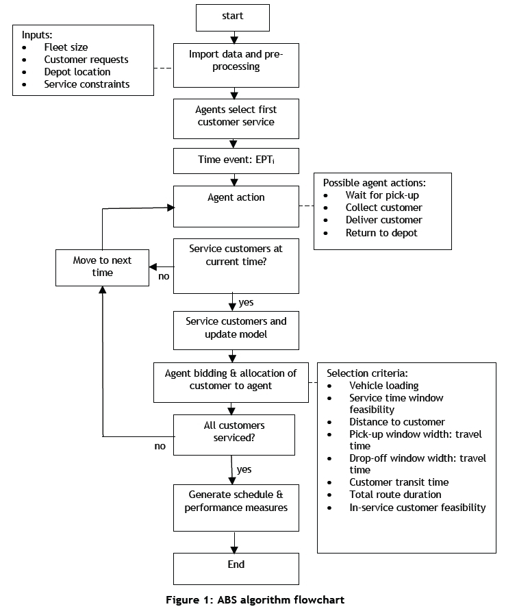
The major steps and decisions the model performs are shown in Figure 1, with the model inputs, agent decision criteria, and possible agent moves also shown.

In the data sets there are two types of customers (i), of equal number, namely:

1. Customers who have specified a desired pick-up time (DPTi) window, where the earliest pickup time (EPTi) and latest pick-up time (LPT) in which they must be serviced is defined.

2. Customers who have specified a desired drop-off (DDTi) time window, where the earliest delivery time (EDTi) and latest delivery time (LDTi) in which they must be serviced is defined.

Since only the pick-up (drop-off) time limits for DPT (DDT) customers are defined, the EDT and LPT (EPT and LDT) are set to 0 and 1440 minutes respectively.

Pre-processing similar to that described by Cubillos et al. [8] was applied. Service time window limits depend on the maximum ride time (MRT) constraint and vehicle servicing time. Pick-up and drop-off time window limits were adjusted accordingly, by setting smaller EDT (EPT) and LDT (LPT) time window limits for DPT (DDT) customers.

Central to the ABS is the 'bidding' process agents use to search for feasible insertions of customers into their schedules. The addition of a customer to an agent's schedule must not violate the service constraints of customers already in transit.

At the start of the model, k agents each select one of n customers (i) to service, based on the ith earliest possible pick-up times (EPTi). Each agent calculates the actual pick-up time (APTi) they should collect a customer, to minimise customer waiting and transit times for the first customer serviced. Once the APTis are known, the agents determine the time they must leave the depot to begin their customer service schedules. The EPTi was chosen as the time event for customer selection to prevent selection bias between DDT and DPT customers. Had EDTi been used, these events would typically occur earlier for DDT customers than DPT customers, following the time window pre-processing modification. An objective function (Z) is not used for the first customer selection as the Z scores would all be the same for all agents, given that they are all starting from a common depot.

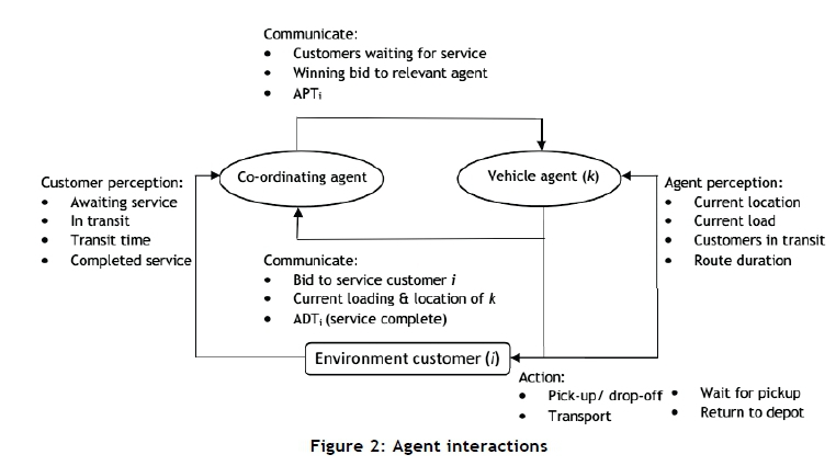
In the ABS, agents progressively build their own schedules as the model moves to pick-up and dropoff time events. Following a drop-off event, all agents are triggered to place bids for the 'cost' of servicing all awaiting customers who have not already been allocated to an agent for servicing. The bids are communicated to a central co-ordinator agent who informs the agent with the lowest bid of customers awaiting the commencement of their service, customers in transit, and the customers who have been serviced. Figure 2 shows the interactions between the vehicle agents, co-ordinating agent, and customers. Depending on the outcome of the bidding process, the agent who has just serviced a customer will perform one of the actions shown in Figure 2. The model moves through discrete time events by going to the next scheduled pick-up time event (APTi) or drop-off event (ADTi), depending on which event occurs first in the progression of time. Note that ADTs are the time the vehicle has completed service at a drop-off location - i.e., the vehicle is ready to leave.

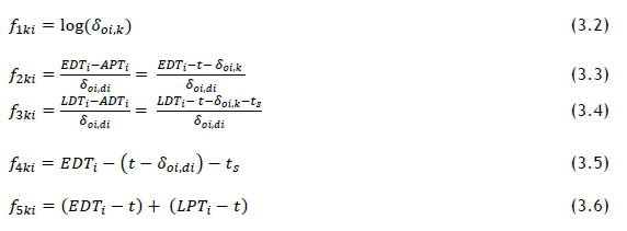
Each agent bids to service customers based on five factors that are combined into a weighted objective function, expressed as a bid (Zki) by agent k to service customer i at the current time in the model:

Factors f1,…,5ki are calculated as follows:

subject to the following conditions:

 

The first factor (3.2) in the objective function (3.1) calculates the Euclidean distance between an agent's current location and the customer's location. In (3.2) the calculated distance is transformed using a lognormal distribution, to ensure customers closest to a vehicle's current location have a lower factor score than customers further away. By using a lognormal distribution, the 'weighting' of this factor in the objective function (3.1) is reduced in the event of large distances between an agent and a potential customer. This enables a higher chance of a feasible bid, if the other factors in the objective function are small in magnitude. If a lognormal distribution were not used, customers with potentially good service windows, but located further away, would obtain a high Zki value, making it unlikely that these customers would be selected for servicing. Factors f_2ki(3.3) and f3ki (3.4) aim to determine the service window 'tightness'. Factor f_2ki(3.3) determines a ratio between the time window of the actual pick-up time and earliest delivery time to the travel time incurred, if the agent were to transport the customer directly from origin to destination. Similarly, factor f_3ki(3.4) determines the ratio between the actual delivery time and latest delivery time window to the direct transit time of a customer. These factors yield a lower score if a customer is serviced between the EDTi and LPTi. The use of these factors also avoids the servicing of customers close to the limits of EPTi and LDTi, as this would result in long transit times. These factors help to ensure that the servicing of customers with tight pick-up windows are picked up as late as possible, whereas customers with tight drop-off windows are picked up as early as possible.

In allocating a customer to a vehicle, the expected customer transit time is considered in the agent bid by factor f4ki (3.5).

To prevent customers with EPTs and LPTs far in advance of the model's current time from being favoured for selection, factor f5ki (3.6) was added to Zki (3.1). During development of the model, in the absence of this factor, it was found that customers located close to an agent's current location were being favoured for selection. This was despite their service times being far in advance of the model's current time, with certain customers not being serviced at all, thus yielding infeasible solutions.

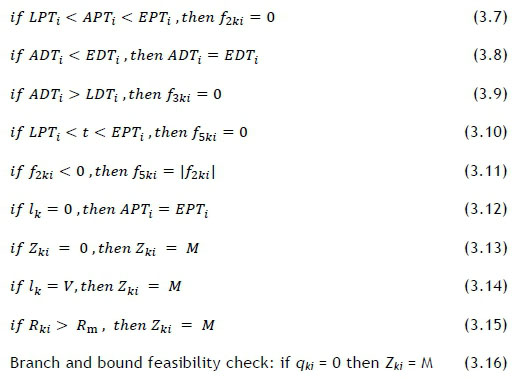
Equations (3.7) to (3.16) are constraints imposed to ensure the time precedence of events, such as ensuring that a pick-up (drop-off) event does not occur after (before) a drop-off (pick-up) event. If a vehicle is empty and it is assigned to service a customer, the APTi is set equal to EPT (3.12) to minimise waiting and transit times.

If Zki (3.1) is found to be infeasible at a bid event, it is set to a large (big M) value (10¹⁰⁰). In the event that all bids are infeasible at the current time in the simulation, the model moves forward one unit in time. Thereafter all vehicle agents re-submit bids to service customers at the new time. The model will continue moving forward one unit in time until either a feasible bid is found or the next APTi or EDTi event occurs. This approach ensures a sequential progression of time during the simulation. It also prevents customers from being skipped for servicing, which would occur if the simulation simply moved to the next APTi or EDTi event.

The feasibility of Zki (3.1) is also dependant on the available vehicle capacity, ensured by equation (3.14).

Equation (3.15) ensures that agents do not exceed the maximum vehicle route duration. Rki is calculated using a sub-function that sums an agent's route duration based on the route duration already incurred by agent k, the route duration to service the customers currently in transit by k, the expected additional route duration for the potential new customer i, and the route duration to return to the depot from the potential new customer's destination. This sub-function assumes that the potential new customer will be serviced last in k's schedule, directly between the customer's origin and destination.

In general, when adding a new customer to an agent's routing schedule, there are four possible route insertion options to be considered, illustrated in Figure 3:

1. Both the pick-up and the drop-off events are inserted at the end of the last schedule block.

2. Both the pick-up and the drop-off events of a customer are inserted between two other successive vehicle stops.

3. The pick-up of a customer takes place somewhere between other scheduled stops, with the customer drop-off taking place at the end of the vehicle's scheduled sequence.

4. The pick-up and drop-off events of a customer are separated by at least one other stop in the vehicle's scheduled sequence.

 

 

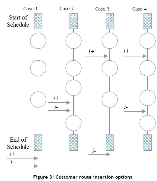
A customer insertion into an agent route can result in the schedule becoming infeasible for cases 2 to 4 in Figure 3. The required servicing time windows of the customers already in transit are not considered in equations (3.7) to (3.15). Therefore a branch and bound sub-function was added to check the servicing feasibility of the customers already in transit when adding a potential new customer to a route. Each time the branch and bound sub-function is run there are (2i)\ possible routing sequences, as each customer has a unique origin and destination. Most of the sequences would be infeasible due to the required time precedence of events (pick-up event before drop-off event). It would be computationally inefficient to conduct a branch and bound search of a fully-loaded six-seat vehicle, since 12! possible routing combinations would have to be considered. Therefore, the branch and bound sub-function determines route feasibility based on the delivery time windows (EDTi and LDTi) only. Given that the customers are already in transit, this results in a maximum of 6! possible routing combinations that must be considered by the agent. The branch and bound sub-function runs until a feasible service schedule is found, or until all routing possibilities have been considered and rejected. It returns a binary value (3.16) indicating whether a feasible route has been found. If so, the new customer is added to the agent's schedule.

The five factors in the objective function are weighted. Setting of the weighting constants can be considered a form of agent training, since they effectively decide how important each factor is in agent decisions. Therefore, good values for the weighted constants were found using a genetic algorithm (GA). The GA used the agent routing algorithm solution cost (total distance travelled) as a fitness function to be minimised using data set Pr08. This data set has six vehicles to service 72 customers, and is similar to the overall average number of vehicles and customers across all the data sets. The ratio of vehicles to customers in Pr08 was relatively low in comparison with the other data sets, making it more difficult to find a feasible solution. The logic was that, if good weights could be found for the function for data set Pr08, and they would yield a low solution cost, these weights would be suitable for all the other data sets.

 

4 OBSERVATIONS, RESULTS AND DISCUSSION

4.1 Observations and results

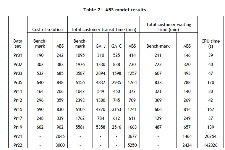
The ABS model obtained feasible solutions for all 22 test data sets. The performance measures obtained for data sets with complete benchmark solutions available are listed in Table 2. Column 'GA_J' shows results from Jorgensen et al. [15] and column 'GA_C' shows results from Cubillos et al. [8].

Short and consistent transit times were obtained for all customers. Pick-up events were found to have been scheduled relatively close to or at the customers' EPTs. Similarly, for the DDT customers, ADTs were scheduled closer to the customers' desired EDTs than their LDTs.

In comparison with the benchmark solutions, the ABS produced a balanced distribution of customers among the three vehicles. Fewer customers needed to share routes between their desired locations. In the benchmark solution schedules, most customers were placed on indirect routes between their transport nodes, resulting in higher total transit times. The benefits of more direct routing of customers are reflected in the short transit times for the ABS model.

The ABS model produced lower customer transit times for all the data sets than those obtained by the other three studies, except for total travel time for Pr01, which was 104 minutes more than Jorgensen et al. [15]. The ABS customer transit times were significantly better than the benchmark times, averaging 67% less than the benchmark values.

The ABS model yielded better total customer waiting times in comparison with the benchmark solutions, for six out of the nine data sets. The ABS produced a consistent ratio of approximately 2.5 minutes of customer transit time incurred for each minute of waiting time across all the data sets. While the ABS model yielded worse customer waiting times for data sets Pr15, Pr17, and Pr19 in comparison with the benchmark values, the total customer transit times obtained by the benchmark solutions were significantly higher than those found using the ABS model. For Pr17 the benchmark solution has a ratio of 13.7 minutes transit time for each minute of waiting time, in comparison with the ABS model ratio of 2.5. Overall the benchmark data sets average a ratio of 7.2 minutes of transit time for each minute of waiting time. This indicates that the benchmark solutions scheduled numerous non-sequential customer pickups and drop-offs on the routes, resulting in higher transit times. This was confirmed by comparing the two schedules produced by the two methods.

The ABS model produced consistent average customer waiting times of about six minutes for all the data sets, including the large data sets Pr21 and Pr22. The benchmark solutions' average waiting times were erratic, varying from less than four to 15 minutes. In a real-world application, the ability of the ABS model consistently to yield the same average customer waiting times would enable customers to be informed in advance of their approximate APTs, given their chosen EPTs.

It is evident that the ABS model developed here provides significantly better customer service, through lower travelling and waiting times than the solutions obtained using conventional operations research methods. The improved customer service is at the expense of higher solution operating costs. In practice, a balance between the amount of waiting and travel time incurred would be desirable. It is clear that the ABS has been able to find a suitable and consistent balance across all the data sets.

As expected, the ABS model produced higher solution costs across all the data sets in comparison with the benchmark values (Table 2) provided by Cordeau and Laporte [7]. This was partly due to better customer service measures in all instances, and partly due to the use of hard time window constraints. The costs incurred were not excessively higher than those of the benchmarks, with an average of 32 per cent higher schedule cost, and, in the worst case (PR19), a maximum of 50 per cent higher schedule cost.

In real-world applications it could be argued that the higher solution costs incurred are worth paying for, given the substantially better customer quality of service that would be provided. This would be scenario-specific and dependent on whether the customer is willing to pay more for the gains in service that would be achieved.

4.2 Computer processing speed

The largest number of customer requests for the data sets provided by Cordeau and Laporte [7] was 144 requests, and they required 6.7 minutes of processing time to obtain a solution. This is reasonable, particularly considering the high-level development environment used for the programming (MATLAB). The ability of the ABS to obtain a solution in a reasonable time makes the method practical for use on a daily basis to schedule vehicle routes. The ABS model yielded similar computational times for all of the data sets with similar numbers of customers.

The design of the ABS algorithm requires each agent to place a bid for all awaiting customers at each time event. This results in an increase in computational time required as the number of agents and customers increases, as was also found by Salamon [20]. The increasing computational time for larger problem sizes imposes a practical limit on the scalability of the model beyond 360 customer requests.

Algorithm processor time profiling showed that a significant portion of computational time was being used by the branch and bound route feasibility sub-function. Currently, the sub-function has been designed to re-initialise if infeasible branches are found, resulting in duplicate computations of route segments. Speed optimisation of this and other computationally-intensive code portions would significantly improve processing time.

The scalability of simulations to obtain solutions for varying problem sizes is an important feature, with a need in practice to solve increasingly large problems that represent the demands of real public transport systems. The ABS model was able to obtain solutions in polynomial time for this NP-hard problem for the larger data sets of Pr21 and Pr22.

4.3 ABS as a general VRP solver

It should be noted that the ABS development and implementation framework used in this work is applicable to any VRP, but will naturally be suited to highly-constrained real-world problems. This is due to small but complex search areas found in such problems. Problems with varying vehicle capacities, tight and hard-time windows, and any problem-specific, additional constraints could be addressed.

In order to apply the method to other VRP problems, the specific functions that agents must carry out need to be developed, and the sequence in which they are applied needs to be defined. Weighting factors for decisions can either be pre-optimised, as done in this work, or modified during algorithm use when applying a learning scheme.

 

5 CONCLUSIONS

An ABS method was developed to solve the DARP. Solutions obtained compare favourably with other published results. The method was shown to be practical for instance sizes up to 360 customers and 35 vehicles. In addition, an ABS development and implementation framework has been presented that can be used to develop solution algorithms to provide good solutions to any VRP, and particularly to highly-constrained, real-world problems.

 

REFERENCES

[1] Savelsbergh, M.W.P. & Sol, M. 1995. The general pick-up and delivery problem, Transportation Science, 29(1) pp 17-29.         [ Links ]

[2] Cordeau, J.F. & Laporte, G. 2007. The dial-a-ride problem: Models and algorithms, Annals of Operations Research, 153(1) pp 29-46.         [ Links ]

[3] Hansen, J.B. 2010. The dial-a-ride problem and exploiting knowledge about future customer requests, Master's thesis, Aarhus University, Denmark.         [ Links ]

[4] Berbeglia, G., Cordeau, J.F, Gribkovskaia, I. & Laporte, G. 2007. Static pick-up and delivery problems: A classification, TOPS, 15(1), pp 1-31.         [ Links ]

[5] Cordeau, J.F. & Laporte, G. 2002. Tabu search heuristics for the vehicle routing problem, Metaheuristic Optimization via Memory and Evolution: Tabu Search and Scatter Search, 30, pp 145-163.         [ Links ]

[6] Cordeau, J.F., Desaulniers, G., Desrosiers, J., Solomon, M.M. & Soumis, F., 2002. VRP with time windows, in The vehicle routing problem, editors Toth, P. & Vigo, D., Society for Industrial and Applied Mathematics, pp 157        [ Links ]

[7] Cordeau, J.F. & Laporte, G. 2003. The dial-a-ride problem (DARP): Variants, modelling issues and algorithms, Quarterly Journal of the Belgian, French and Italian Operations Research Societies, 1(2) pp 89-101.         [ Links ]

[8] Cubillos, C., Urra, E. & Rodriguez, N. 2009. Application of genetic algorithms for the DARPTW problem, Int. J. of Computers, Communications & Control, IV(2), pp 127-136.         [ Links ]

[9] Baugh J.W., Kakivaya, G.K.R. & Stone, J.R. 1998. Intractability of the dial-a-ride problem and a multi-objective solution using simulated annealing, Engineering Optimization, 30(2), pp 91-123.         [ Links ]

[10] Cordeau, J.F. 2006. A branch-and-cut algorithm for the dial-a-ride problem, Operations Research, 54, 573-586.         [ Links ]

[11] Zidi, I., Mesghouni, K., Zidi, K. & Ghedira, K. 2012. A multi-objective simulated annealing for the multi-criteria dial a ride problem, Engineering Applications of Artificial Intelligence, pp 1121-1131.         [ Links ]

[12] Fu, L. 2002. Scheduling dial-a-ride paratransit under time varying, stochastic congestion. Transport Research B-Methods, 36, pp 485-506.         [ Links ]

[13] Cordeau, J.F., Gendreau, M., Hertz, A., Laporte, G. & Sormany, J.S. 2004, New heuristics for the vehicle routing problem, Logistics Systems: Design and Optimization, 2005, pp 279-297.         [ Links ]

[14] Cordeau, J.F., Laporte, G., Savelburgh, M.W.P. & Vigo, D. 2007. Vehicle routing, in Transportation, Handbooks in Operation Research and Management Science, 14, pp 367-428.         [ Links ]

[15] Jorgensen, R.M., Larsen, J. & and Bergvinsdottir, K.B. 2007. Solving the dial-a-ride problem using genetic algorithms, The Journal of the Operational Research Society, 58 (10), pp 1321-1331.         [ Links ]

[16] Segfried, R., Lehmann, A., Khyanari, R.E.A. & Kiesling, T. 2009. A reference model for agent-based modelling and simulation, Proceedings of the 2009 Spring Simulation Multi-conference, Article 23.         [ Links ]

[17] Zeddini, B., Temani, M., Yassine, A. & Ghedira, K. 2008. An agent-oriented approach for the dynamic vehicle routing problem. International Workshop on Advanced Information Systems for Enterprises, pp 7076.         [ Links ]

[18] Vokrinek, J., Komenda, A. & Pechoucek, M., 2010. Agents towards vehicle routing problems, Proc. of 9th Int. Conf. on Autonomous Agents and Multi-agent Systems (AAMAS).         [ Links ]

[19] Barbucha, D. & Jedrzejowicz, P. 2007. An agent-based approach to vehicle routing problem, International Journal of Applied Mathematics and Computer Science, 4(1), pp 18-23.         [ Links ]

[20] Salamon, T. 2011. Design of agent-based models. Zivonin: Tomas Bruckner.         [ Links ]

[21] Cordeau, J.F., Gendreau, M. & Laporte, G. 1997. A tabu search heuristic for the static dial a ride problem. Transport Res B-Meth, 37, pp 579-594.         [ Links ]

 

 

Available online 11 Nov 2016

 

 

Presented at the 45 annual conference of the Operations Research Society of South Africa (ORSSA) held from 11-14 September 2016 in Stellenbosch, South Africa
* Corresponding author Ian.campbell@wits.ac.za
# The author was enrolled for an MSc Eng (Industrial) degree in the School of Mechanical, Industrial & Aeronautical Engineering, University of the Witwatersrand