GENERAL ARTICLES

 

Optimisation of radio transmitter locations in mobile telecommunication networks

 

 

T. Schmidt-Dumont^#; J.H. van Vuuren^*

Department of Industrial Engineering, Stellenbosch University, South Africa

 

 

---

ABSTRACT

Multiple factors have to be taken into account when mobile telecommunication network providers make decisions about radio transmitter placement. Generally, area coverage and the average signal level provided are of prime importance in these decisions. These criteria give rise to a bi-objective problem of facility location, with the goal of achieving an acceptable trade-off between maximising the total area coverage and maximising the average signal level provided to the demand region by a network of radio transmitters. This paper establishes a mathematical modelling framework, based on these two placement criteria, for evaluating the effectiveness of a given set of radio transmitter locations. In the framework, coverage is measured according to the degree of obstruction of the so-called 'Fresnel zone' that is formed between handset and base station, while signal strength is modelled taking radio wave propagation loss into account. This framework is used to formulate a novel bi-objective facility location model that may form the basis for decision support aimed at identifying high-quality transmitter location trade-off solutions for mobile telecommunication network providers. But it may also find application in various other contexts (such as radar, watchtower, or surveillance camera placement optimisation).

---

OPSOMMING

Verskeie faktore moet in ag geneem word wanneer radiosender-plasingsbesluite deur mobiele telekommunikasienetwerke gemaak word. In die algemeen word area-oordekking en gemiddelde seinsterkte in hierdie besluite as belangrike kriteria geag. Hierdie kriteria gee aanleiding tot 'n twee-doelige fasiliteitplasingsprobleem gemik op die soeke na aanvaarbare afruilings tussen die maksimering van totale area-oordekking en die maksimering van gemiddelde seinsterkte aan gebiede waarin aanvraag na oordekking bestaan. 'n Wiskundige modelleringsraamwerk, gebaseer op hierdie twee plasingskriteria, word in hierdie artikel vir die evaluering van 'n versameling radiosenderliggings daargestel. In die raamwerk word oordekking gemeet volgens die mate waartoe die Fresnel-sone tussen die handtoestel en die basisstasie belemmer is, terwyl seinsterkte aan die hand van radiogolf-voortsettingsverliese gemodelleer word. Hierdie raamwerk word gebruik om 'n nuwe, twee-doelige fasiliteitplasingsmodel te formuleer wat as basis kan dien vir besluitsteun in die soeke na hoë-kwaliteit senderliggingsafruilings deur mobiele telekommunikasie-netwerkverskaffers, maar vind ook toepassing in verskeie ander kontekste (soos die optimale plasing van radars, uitkyktorings, of waarnemingskameras).

---

 

 

1 INTRODUCTION

Mobile telecommunication has revolutionised the modern world. It has become an absolute priority for mobile telecommunication network providers to cover as much area as possible in their service provision. Currently, network providers have the choice of using a combination of second generation (2G), third generation (3G), or fourth generation (4G) networks for their service provision.

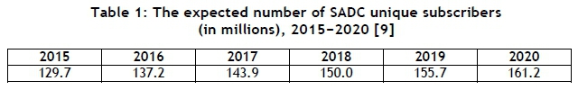
The choice of the type of network and the resulting placement of radio transmitters forming the network are of primary importance to network providers, especially when taking into account the prospective growth of smartphone users in Africa. Reed et al. [19] state that "... the number of smartphone connections will rise from about 79 million at the end of 2012 to 412 million by 2018, according to forecasts by Informa". But it is not only the number of new smartphone connections that is expected to achieve such impressive growth; 2G networks and feature phones are expected to remain a key aspect of mobile networks in Sub-Saharan Africa where, due to the relatively low gross domestic product (GDP), smartphones remain beyond reasonable levels of affordability for a large portion of the population. The expected growth in the number of unique mobile subscribers in the Southern African Development Community (SADC) countries during the period 2015-2020 is shown in Table 1. This will especially be the case in semi-urban and rural areas where new mobile networks are established [9].

In a country as large as South Africa, the effective placement of radio transmitters aimed at providing a high-quality mobile network service presents a major challenge. As a result, the placement of radio transmitters is constantly debated. Multiple factors have to be taken into account when new radio transmitter placement decisions are made. The focus in this paper, however, will be on the area that a network of radio transmitters is able to cover, and on the quality of this coverage. Although the total area covered by the network is usually of prime importance, the average signal level provided to covered areas is also of considerable interest - especially in densely-populated urban areas - since this will maximise the quality of service provided. These considerations naturally result in a bi-objective facility location problem where the goal is to achieve an acceptable trade-off between maximising both the total coverage and the average signal level achieved by a network of radio transmitters. These objectives are in conflict, in the sense that placing transmitters far apart tends to increase their coverage, while placing them closer together tends to increase the average signal level they provide.

The area that can be covered by a radio transmitter depends on three main factors: the power of the transmitter, the type and configuration (antenna height and beam direction) of the antenna installed at the transmitter, and the topography and land cover of the surrounding area [14].

Radio transmission generates an infinite family of nested ellipsoids of electromagnetic waves, called Fresnel ellipsoids, with the transmitter and receiver at their foci. For effective radio transmission, the innermost of this family of ellipsoids, called the Fresnel zone, should be sufficiently unimpeded [11]. The area that may be considered covered by a radio transmitter therefore includes all those potential handset receiver points on the earth's surface for which the Fresnel zones between the transmitter and the points in question are sufficiently unimpeded.

The objective in this paper is to design and demonstrate the working of a flexible, computerised decision support framework capable of suggesting high-quality placement alternatives for a network of radio transmitters in rural areas that achieves suitable trade-offs between the conflicting objectives of maximising network area coverage and maximising the average signal level provided to the covered areas. This framework is based on a bi-objective combinatorial optimisation modelling approach, and is applicable to cellular telephone transmission towers operating with 2G technology. The methodology used to establish this framework is, however, not restricted to mobile communication networks. It could be easily adapted for various other applications, including facility location of radar towers in a military context, fire-lookout watchtowers, anti-poaching observation cameras in a nature conservation environment, or surveillance cameras for securing industrial plants.

The paper is organised as follows. After conducting a brief review of the literature related to radio transmitter location decision support in §2, we present our bi-objective framework in §3 for the evaluation of a set of radio transmitters on a given portion of the earth's surface. This is followed in §4 by the formulation of a mathematical model, based on the framework of §3, for optimising radio transmitter locations. In §5 this model is incorporated into the design of a user-friendly decision support system for radio transmitter location. The effectiveness of this decision support system is demonstrated in §6 by applying it to a real case study. The paper closes in §7 with a brief conclusion and some ideas about possible future work.

 

2 LITERATURE REVIEW

This section is devoted to a brief review in §2.1 of the literature related to facility location models that have been used in the planning of radio transmission networks. The focus shifts in §2.2 to wave propagation and various parameters that have an influence on radio communication over different types of surfaces. The section closes in §2.3 with a discussion of those data required to generate an instance of the bi-objective radio transmitter location problem described in the introduction.

2.1 Models for radio transmitter location

In second generation mobile telecommunication networks, the network planning problem may be decomposed into two distinct phases: (offline) coverage planning which involves antennae placement to achieve maximum service coverage, and (online) capacity planning which involves frequency assignment planning [1]. The coverage planning problem has generally been modelled using variations on the celebrated set covering problem, as discussed by Daskin [5]. Amaldi et al. [1] describe this problem, known in the context of radio transmitter network planning as the coverage problem, as follows: "Given an area where service provision has to be guaranteed, determine those locations where radio transmitters should be placed and specify their configurations such that each point (or user) in the service area receives an adequate signal level". Two main modelling approaches have been adopted in the literature to solve instances of the coverage problem [1].

In continuous optimisation models, a specified number of base stations are to be located at any site within a given space to be covered, where the antennae co-ordinates are the continuous variables of the problem. This space may exclude certain forbidden areas in which no transmitter placements are possible. In certain cases other parameters, such as the antennae orientations and/or the transmission power, may also be considered as variables. Amaldi et al. [1] claim that the most important element of this type of optimisation model is the propagation prediction model used to estimate the signal intensity at each point in the coverage area. Various functions have been proposed over the years for signal estimation. These range from simple empirical models such as those developed by Hata [10], to more sophisticated ray-tracing methods such as that proposed by Iskander and Yun [12].

The objective function of the coverage problem is usually determined by some measure of the quality of service, such as the largest minimum signal intensity at any location [1]. Due to the high complexity of propagation loss functions, global optimisation techniques are usually employed to tackle these problems, as illustrated by Sherali et al. [21], who employ a linear combination of a 'minisum' objective and a 'minimax' objective. The former objective is to minimise the sum of all the weighted path loss predictions in the design space along with a penalty term that represents a path loss greater than a specified threshold value for a specific demand point. The latter objective is to minimise the maximum of all the weighted path loss predictions, again including a penalty for exceeding the maximum acceptable path loss.

A convex combination of the above-mentioned objective functions is often used to take advantage of the respective merits of each of the objective functions while minimising their drawbacks. The resulting model accommodates two types of design constraints. The first is treated as a 'soft' constraint, ensuring that each receiver location in the design space receives an adequate signal level. This constraint is incorporated into the model by a penalty term in the minisum objective. The second constraint type restricts the transmitter placement location to specified acceptable subsets of the design space.

The second coverage problem modelling approach involves the use of discrete mathematical models [1]. In discrete optimisation models, a number of test sites or demand nodes representing potential users of the network have to be identified from a predetermined set within the service area. Instead of allowing base stations to be placed at any location in the coverage area, discrete mathematical models restrict the positioning of these base stations to a set of so-called 'candidate' sites. In these models, the area covered by each base station is determined a priori, generally using a radio wave propagation predictor and taking the surrounding topology and morphology of the terrain into account [16]. The area covered by a base station located at a candidate site is therefore assumed to be known in such an optimisation model.

Krzanowski and Raper [14] explain that in both the continuous and the discrete modelling paradigms, total cover problems require the determination of the minimum number of facilities in order to meet all the demand. In contrast, partial cover problems arise when the number of facilities to be placed is fixed, and their locations have to be chosen in order to maximise the demand that can be covered using the limited number of facilities. A further extension of the partial cover problem is the so-called general cover problem, in which the objective is to minimise the maximum distance between a facility and the demand points it covers. Mathar and Niessen [16] demonstrate how the coverage problem is an extension of the classic minimum cost set covering problem [5].

It is often the case, however, that due to limitations on the installation cost, the covering requirement is treated as a 'soft constraint', and as a result the problem requires a trade-off between maximising coverage and containing installation cost.

As Amaldi et al. [1] point out, one problem in these models is that they do not take overlaps between cells (the areas covered by specific base stations) into account. This becomes very important later during the frequency allocation phase of capacity planning when dealing with handover (i.e., the possibility of a user remaining connected while moving from one cell to another). To overcome this shortcoming, cell boundaries may be established during the network planning phase by introducing variables that explicitly assign demand nodes to base stations. An example of this is provided by Amaldi et al. [1].

Due to the large dimensions of the optimisation problems typically involved in radio transmitter facility location planning problems, metaheuristics are often employed as approximate optimisation techniques instead of pursuing exact model solutions. Simulated annealing has, for example, been used by Mathar and Niessen [16] in an instance where the complexity of the optimisation problem places an optimal solution beyond the reach of current computing technology. Krzanowski and Raper [14] instead used a hybrid genetic algorithm designed to take the surrounding geography into account during the site selection process.

2.2 Requirements for effective radio transmission

Radio wave propagation loss is perhaps the most important factor influencing effective radio transmission. Iskander and Yun [12] define propagation loss at a point r as "the ratio of transmitted power P_t(r₀) at r₀over the received power P_t(r) at r". In free space, the propagation loss, in dB, can be simply expressed as

where G_tand G_rare the gains of the transmitting antennae and the receiving antennae respectively; D is the distance between the transmitter at r₀and the receiver at r; and λis the wavelength in free space [12]. The standard relationship ƒ·λ = ν holds between the frequency ƒ and wavelength λof radio waves, where νdenotes the speed of the radio waves in free space. In order to ensure effective radio wave transmission, the propagation loss in (1) must remain below a specified threshold value to provide a signal of the required intensity [21].

Studies conducted in the San Francisco Bay area by Feuerstein et al. [7] have shown an increased radio wave propagation loss when the Freznel zone, described in the introduction, is partially obstructed.

Various models have been proposed to determine propagation loss between two points in obstructed space. These propagation loss prediction models may be divided into three different categories: empirical, theoretical, and site-specific models.

Empirical models are developed by taking extensive field measurements, from which the equations are then derived. Due to variations in the surrounding environment, however, such empirical models may lack accuracy when applied to an area that is different from the area where the measurements on which the formulae are based were made. Empirical models are generally used for propagation predictions in macrocells that have radii ranging from 1 km to 30 km [15]. The advantage of using empirical models is that they are simple and efficient [12]. Site-specific models, such as the ray-tracing model introduced by Seidel and Rappaport [20], are based on very detailed numerical analyses, and as a result require detailed and accurate input parameters - including data on the specific locations of buildings, their heights, and the distances between the walls of these buildings. These models are generally used in urban areas when propagation predictions are made for microcells with radii of up to 1 km or for picocells with radii of up to 500 m [15]. The disadvantage of using site-specific propagation models is the large computational overhead that may even be beyond the current capability of computers [12].

Theoretical models are derived from the underlying physics, but are based on the assumption of ideal conditions. As a result, they typically achieve a middle ground between the accuracy of site-specific models and the computational efficiency of empirical models [12]. In Europe, research efforts in respect of propagation prediction models are promoted by the European Cooperation in the Field of Scientific and Technical Research (COST), which is "an open, flexible framework for research and development cooperation between universities, industry and research institutions" [8].

One aim of the so-called COST 231 action has been to elaborate on powerful prediction models, many of which have now become widely accepted. These include extensions to Hata's empirical model [10], which addresses several shortcomings of the original model proposed by Hata, such as the so-called COST 231 -Hata Model and the COST-231 -Walfisch-Ikegami Model [8]. For example, the COST 231 - Hata Model takes the frequency ƒ, the distance between the antennae D, the base station antenna height h_b, and the mobile antenna height h_minto account. Then, as outlined by Kürner [15], the COST 231-Hata Model yields the basic propagation loss

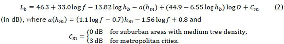
The COST 231-Hata Model is restricted to the following range of parameters: ƒє [1500,2000] MHz, h_bє[30,200] m, h_m є [1,10] m, and D є[1,20] km. The model is further restricted to use in macrocells. Also, the base station antennae heights must be above the roof-top levels of the buildings adjacent to the base station for the model to yield accurate results.

2.3 Data required for radio transmitter location decisions

When placing radio transmitters, the complex distribution of expected demand patterns for the service to be provided, the presence of area-specific geographic features - such as topography, morphology, and the type of land cover - and the technological aspects and capabilities of the network have to be taken into account simultaneously [14]. The service area for the network and information on possible locations for the placement of the transmitters also has to be known. Krzanowski and Raper [14] propose the use of geographic information systems (GISs) to obtain the required information about the topography, morphology, and the land cover for the area under consideration. GIS is a technology designed specifically to handle environmental and spatial information with great accuracy.

In the models discussed in §2.1, demand plays a crucial role in the facility location process. It is, however, not as easy to obtain expected demand values as it is to acquire environmental information. Measuring demand has become increasingly important as mobile radio communication has become a mass communication technology. As a result, demand coverage may be converted to monetary terms and viewed as revenue coverage [26]. This has led to the development of the demand node concept (DNC), established by Tutschku and Tran-Gia [27], which is a discrete population model for expected mobile traffic description. The DNC represents the spatial distribution of the expected demand at discrete points, known as demand nodes. Each demand node represents a fixed quantum of demand, usually accounted for by a fixed number of call requests per unit time. Based on the land use of an area, the spatial traffic distribution may be derived using complex estimation methods, and be stored in a traffic matrix. From this traffic matrix, the demand nodes may then be generated using a clustering method [26].

Krzanowski and Raper [14] describe a similar method to estimate expected demand, calculated as the weighted sum of vehicular traffic, population density, and the business counts in the area of interest. Each of these factors contributes to the resulting traffic layer, which is a direct input to their hybrid genetic algorithm for transmitter location in wireless networks.

 

3 RADIO TRANSMITTER LOCATION QUALITY EVALUATION

This section is devoted to the establishment of a suitable framework to evaluate the effectiveness of a given set of placement locations for a network of 2G mobile telecommunication radio transmitters. The focus in §3.1 is on the line of sight between a single transmitter and a potential set of receivers, and on the Fresnel zone generated by the electromagnetic waves of the radio communication between these locations. In §3.2, the focus shifts to the propagation prediction model used to ensure that the potential receiver demand points receive an adequate signal level from a single transmitter in order to be considered covered. §3.3 is devoted to an explanation of two performance measures, according to which the quality of a network of transmitter placement locations may be evaluated.

3.1 Modelling area coverage of a single transmitter

The decision support framework developed in this paper for radio transmission tower placement is based on a discrete facility location modelling approach, as discussed in §2.1. The input data to determine radio transmission coverage of an area by a given set of transmitters is a matrix of entries. These correspond to a rectangular grid of placement candidate sites on the earth's surface (which are also the coverage demand points), and contain terrain elevations above sea level for some specified area of interest. For a demand point in this area to be considered covered by a potential transmitter, a relatively unimpeded Fresnel zone should exist between the transmitter and the demand point, as discussed in §1.1. Bresenham's well-known line drawing algorithm [17] is widely used in computer graphics to determine which pixels need to be coloured when drawing straight lines on screen displays. This algorithm can be used to determine those entries in the above-mentioned matrix that form the line of communication between the transmitter and receiver locations under investigation. A complete and accessible description of Bresenham's line drawing algorithm is outlined by McKinney and Agarwal [17].

The axial radius of revolution around the line segment connecting the foci of the first Fresnel ellipsoid at any point ρ on the surface of the ellipsoid between the transmitter and receiver is given by

where d₁represents the distance along the line of visibility between ρ and the transmitter, d₂ represents the distance along the line of visibility between ρ and the receiver, D = d₁ + d₂is the total distance between the transmitter and receiver, and λrepresents the wavelength of the transmitted signal. The distances d₁, d₂and D in (3) may be approximated using the theorem of Pythagoras in cases where the elevations of the transmitter and receiver differ. These parameters are illustrated graphically in Figure 1.

The test for a sufficiently unimpeded Fresnel zone is performed by considering the equation of the straight line of visibility between the transmitter and the demand point, and comparing the lowest point of the first Fresnel ellipsoid and the heights of points on the terrain surface along the line determined by Bresenham's line drawing algorithm. A parameter a e [0,1] is introduced as a user-scalable measure of the required extent to which the Fresnel zone should be unimpeded. Only if the elevation of the lowest point on the first Fresnel ellipsoid, multiplicatively scaled by the parameter a, between transmitter candidate site i and demand point j is higher than the elevation above sea level for all surface points above the line determined by the Bresenham line drawing algorithm between i and j, can the demand point be considered covered in terms of communication feasibility by the transmitter candidate site.

In this way the area of demand points covered by a transmitter placed at a given location can be determined, and a so-called view shed plot may be associated with the transmitter placement. A view shed is a graphical representation that distinguishes between the areas for which the Fresnel zones - with one focus at a transmitter location and the other foci at the various demand points on the earth's surface - are sufficiently unimpeded (i.e., the areas that can be covered by the transmitter) and the areas that the transmitter is unable to cover.

One measure of the quality of a transmitter placement is the percentage of the demand it is able to cover, weighted by importance values assigned to satisfying demand at each demand point. Let J = {1,···, n] denote the set of transmitter candidate locations and receiver (demand) locations. A coverage importance value c_j- is associated with each demand node j e J. The percentage of the demand covered by a transmitter location is simply calculated as the sum of the coverage importance values c_j- of the demand nodes covered by a transmitter, divided by the sum of the coverage importance weightings c_jfor all j e J.

Consider, for example, the portion of terrain shown in Figure 2(a) with latitude and longitude distances between two successive grid points of approximately 308 m and 256 m, respectively.

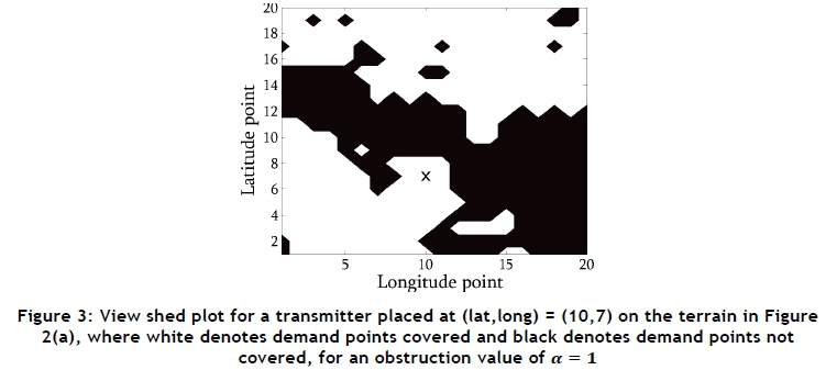
Suppose that demand importance weightings in Figure 2(b) are assigned to the demand points in this area. Then the view shed in Figure 3 results for a radio transmitter placed at the cross located at (lat, long) = (10,7) for the values ƒ = 1 800 MHz, h_b= 50 m, h_m= 2m and a = 1.

It follows that demand covered, weighted by the demand importance values in Figure 2(b), can be determined as 58.41 per cent for a transmitter placed 50 m above the ground at (lat,long) = (10,7) on the terrain in Figure 2(a) if potential demand points are 2 m above the terrain surface, radio waves of 1 800 MHz are transmitted, and the entire Fresnel zone is required to be unimpeded for effective radio communication.

3.2 Modelling signal strength of a single transmitter

An empirical approach to signal propagation prediction is adopted in this paper, since the focus here is on macrocells, in which the type of land cover is only roughly known. More specifically, the propagation loss model selected for use in this paper is the COST 231-Hata Model (2) discussed in §2.2.

The frequency ƒ and antennae height parameters h_band h_mare specified by the user and are thus input parameters to the model. The distance D between the transmitter at candidate site i and receiver at demand point j is the same as that used for the calculation of the axial radius of the Fresnel zone discussed in §3.1, as illustrated in Figure 1. Since all the parameters are known, the resulting predicted radio signal propagation loss can be determined according to (2). The predicted propagation loss L_b(i, j) at a receiver located at demand point j can therefore be subtracted from the transmitted signal strength at a transmitter located at candidate site i to measure the actual signal level at the receiver. The transmitted power Pj. can be converted to units of dBm, a decibel representation of milliwatts, according to the transformation

described by Weisman [28]. A minimal threshold signal level S_minrequired to guarantee a sufficient quality of radio communication also has to be specified by the user, and is usually also given in dBm.

Since the signal level at each of the locations of the grid of demand points can now be calculated, the average signal level provided to the demand points is simply calculated as the sum of the signal levels at each of the covered demand points (i.e., those demand points with an importance rating Cj > 0 that receive an adequate signal level) divided by the number of covered demand points.

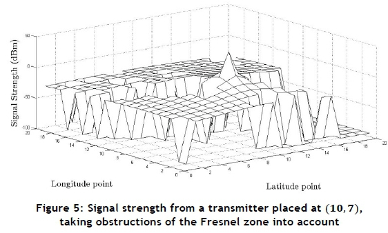
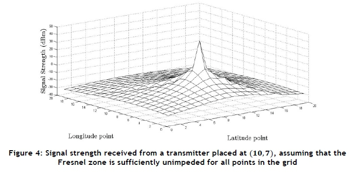
If, for example, ƒ= 1 800 MHz, h_b = 50 m, h_m = 2 m, P'_t- = 20 W and S_min = -95 dBm, then the transmitted power can be calculated as P(t) = 10log(1000 P_t') = 43.01 dBm. Assuming that the Fresnel zone is sufficiently unimpeded at each demand point, the signal level provided to each point in the demand area may be calculated according to (2). The resulting signal level is shown graphically in Figure 4.

If, however, the signal level is only calculated for those demand points in the grid for which the Fresnel zone is sufficiently unimpeded by the terrain in Figure 2(a), as determined using a value of a = 1, the signal level in Figure 5 results. In this figure, any grid point for which the Fresnel zone is not sufficiently unimpeded has been assigned a signal level of -95 dBm. The normalised average signal level provided to those locations with an importance value C_j> 0 may then be calculated as 55.46 per cent.

 

 

3.3 Modelling the combined performance of a network of transmitters

Suppose the locations of a collection of transmitters in a mobile telecommunication network are captured by a binary decision vector x= [₁ -,x_n]^T, where

Then the degree to which transmission demand is actually satisfied by the transmitter placement decision embodied in the vector xabove, weighted by the importance values associated with demand satisfaction at the various receiver locations, is given by

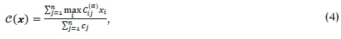
where

Note that double-counting of demand satisfaction importance values is prevented by the maximum operator in (4). This operator is included in (4) to ensure that if demand point j є J is covered by k transmitters, then the importance value c_j, of §3.1 will not be accounted for k times in C(x). This prevention of double-counting is desirable, because it is envisaged that if the performance metric C(x) is used as a maximisation objective when seeking a good placement decision vector x, a large value of C(x) should be achieved by covering as many different demand points as possible instead of focusing on coverage of a cluster of points with high coverage importance values, which may be covered multiple times to achieve a large value for the performance metric C(x).

The degree to which transmission signal quality is actually achieved by the transmitter placement decision embodied in the decision vector xis given by

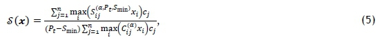
where

The absolute value of the minimum requirement value S_minis added to the signal level in (6) to ensure that the matrix S^a,Pt,Smincontains non-negative entries. The non-negative nature of the matrix is desirable when the performance measure of the average signal level in a covered demand region is computed, as it results in a simplification of the calculation of an appropriate average signal level performance metric. The addition of S_minwill not negatively influence the value of the performance metric, since the performance metric is merely normalised in this way. The reason for taking the maximum over i in (5) is that the strongest signal level achieved from any transmitter i at demand point j should be incorporated into the performance metric S(x). Note that, as in the performance metric C(x) in (4), no double-counting occurs in the summations of (5).

 

4 MATHEMATICAL MODEL

Based on the framework of the previous section, a bi-objective combinatorial optimisation model for radio transmission tower placement is formulated in this section. The model forms the basis for the decision support system developed in the next section.

4.1 Mathematical model formulation

In view of the discussion in §3, a good placement of no more than k radio transmitters is one that achieves a suitable trade-off between

and

subject to the constraints

In (7)-(10), the symbols have the same meanings as in §3. Constraint (9) restricts the number of transmission towers placed to a maximum of k, while constraint set (10) enforces the binary nature of the decision variable vector χ= [x₁, ..., x_n]^T. Since objectives (7) and (8) are conflicting, no single optimal solution to (7)-(10) typically exists. Pareto optimal (trade-off) solutions to (7)-(10) should be pursued instead.

A vector x= [x_1t -,x_n]^Tsatisfying (9)-(10) is called a feasible solution of (7)-(10). A feasible solution xof (7)-(10) dominates another feasible solution x' of (7)-(10) if the inequalities C(x) > C(x') and S(x) > S(x') both hold, and at least one of the inequalities C(x) > C(x') or S(x) > S(x') also holds. A feasible solution of (7)-(10) is Pareto-optimal if no feasible solution of (7)-(10) exists that dominates it [29]. The Pareto front of (7)-(10) is the set of all the objective function vectors corresponding to Pareto-optimal solutions of (7)-(10).

4.2 Solving the mathematical model by simulated annealing

The high computational complexity associated with solving the model (7)-(10) places a brute-force model solution out of reach of current computation technology for realistically-sized problem instances. A more intelligent exact solution approach than a brute-force approach may involve the pre-computation of the quality of demand satisfaction values C_ij^aand the quality of signal strength values S_ij^a,Pt,Smin used in the computation of the objective functions (7) and (8), followed by a binary programming model solution approach employing, for example, the standard branch-and-bound method [29]. In such an approach, the bi-objective model's nature may be accommodated by constraining one of the objective functions to some level β e (0,1) at the most, and solving the single-objective problem with the remaining objective function maximised. This process may be repeated for various values of βin order to trace out the Pareto front in objective space. The anticipated disadvantages of this approach are two-fold: it may take long to solve a single-objective iteration by the branch-and-bound method, and the number of iterations required to trace out a Pareto front of suitable resolution may be large. These disadvantages may be alleviated to some extent by employing an advanced solution technique from the realm of combinatorial optimisation, such as Benders decomposition [4]; but even such a sophisticated solution approach is expected to require long computation times for realistically-sized problem instances.

An approximate solution methodology is therefore employed in this paper to solve the model (7)-(10). Various (meta)heuristics (such as a local search heuristic, the method of tabu search, and the method of simulated annealing) were considered for this purpose. Of these, the method of simulated annealing (SA) was selected due to its flexibility, its small set of parameters requiring user-specification, and its ease of implementation. For a description of the working of SA in the context of single-objective maximisation, the reader is referred to Kirkpartick et al. [13]. The necessary extensions required for multi-objective maximisation are described by Smith et al. [23]. We used the energy difference method of Smith et al. [22] for archiving, generated a first current solution to (7)-(10) randomly to initiate the SA search, and selected an initial temperature according to the average increase method suggested by Busetti [2] and Triki et al. [25]. We also implemented the search epoch protocol described by Busetti [2] with epoch lengths chosen according to the rule of thumb proposed by Dreo et al. [6].

For the local search move operator that was employed, the neighbourhood of a feasible solution of (7)-(10) consists of all those feasible solutions of (7)-(10) that may be obtained by exchanging any one of the transmitter locations with one of its eight neighbouring grid points while keeping the locations of the remaining k- 1 transmitters unchanged. A search move was performed by selecting an element of this neighbourhood according to a uniform distribution as the new current solution. These moves are performed until three successive epochs have elapsed without encountering a solution of (7)-(10) selected for archiving.

 

5 DECISION SUPPORT SYSTEM

This section is devoted to a description of the development and implementation of a DSS that combines the bi-criterion framework for evaluating a set of given transmitter locations (described in §3) with the bi-objective facility location model and the SA approximate solution methodology (described in §4) to create a user-friendly decision support tool for radio transmission tower placement.

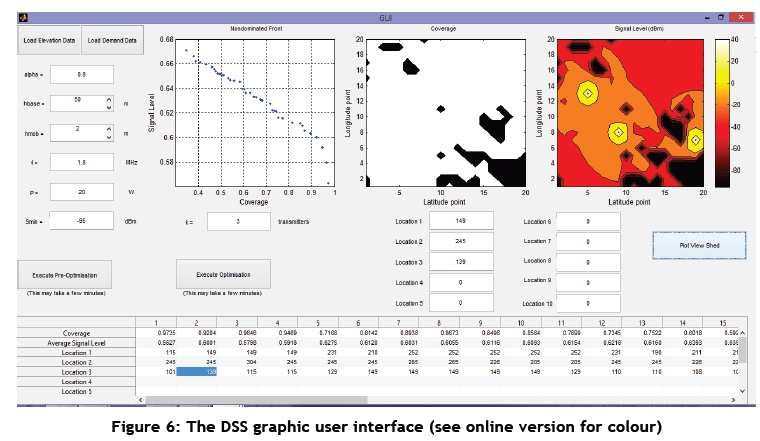
The primary design requirement for the graphic user interface (GUI) of the DSS was to enable the user easily to load the elevation and demand data for an instance of the transmitter location problem into the system, thereby facilitating access to the bi-criterion framework (described in §3) and to the model and solution methodology (described in §4) by non-mathematically inclined users. These data may be loaded into the DSS by clicking the corresponding Load Elevation Data and Load Demand Data buttons in the top left corner of the GUI (Figure 6), after which a Windows Explorer window appears that allows the user to browse for and select the correct files.

The GUI then allows the user to enter the network-specific parameters of the facility location problem instance. These parameters include the scalable parameter to determine the extent to which the Fresnel zone should be unimpeded; the base station and mobile antennae heights h and h respectively; the frequency at which the network will be transmitting; the transmitted power P_t' at the base stations; and the threshold minimum signal level S_minat the top left of the GUI. Thereafter, the pre-optimisation processing phase can be initiated by clicking the Execute Pre-Optimisation button.

Once the pre-optimisation phase is complete, the user may choose the number of transmitters that are to be located, and then initiate the optimisation phase by clicking the Execute Optimisation button. The approximate Pareto front is also displayed on the set of axes towards the top left side of the display, representing objective function space. The performance measures ( ) and ( ) corresponding to this approximation set are displayed, together with the associated set of transmitter grid locations in the table at the bottom of the screen.

The user can then enter any of these sets of transmitter locations into the text boxes labelled 'Location 1' to 'Location 10' towards the middle right of the screen, and prompt the DSS to display the view shed (coverage) and a heat map of the average signal level achieved by the set of transmitter locations. The view shed plot is then displayed on the central set of axes, while the heat map of the average signal level achieved is displayed on the set of axes in the top right corner of the screen.

 

6 REALISTIC CASE STUDY

To assess the quality of the transmitter placement locations suggested by the DSS, comparison with the existing network of an actual local mobile telecommunication network provider - referred to here as network provider 1 - is conducted in this section.

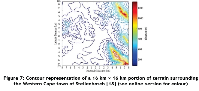
A contour representation of the elevation data for an area surrounding the town of Stellenbosch in the Western Cape Province of South Africa is shown in Figure 7. The area consists of a 16 km x 16 km portion of land stretching from S 33° 51' 20" to S 34° 00' 00" and from E 18° 45' 48" to E 18° 56' 12". This area includes Stellenbosch, whose central coordinates are located at S 33° 53' 12" and E 18° 51' 36", and the outskirts of Cloetesville, Welgevonden, Idas Valley, and Kleingeluk.

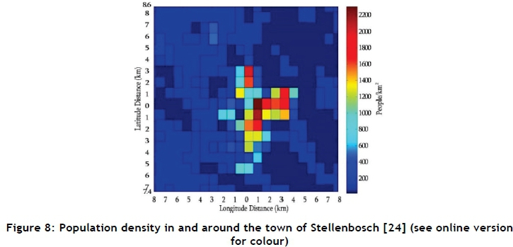
Because of the unavailability of mobile telecommunication coverage importance data (due to their sensitive nature), these data are approximated by the spatial census data shown in the form of a density plot in Figure 8. The resolution of these surrogate coverage importance data are measured as the number of people resident per square kilometre. As seen from Figure 8, the central part of Stellenbosch has a relatively high population density (in excess of 2000 people per square kilometre), which fades away towards the Stellenbosch winelands.

The use of spatial census data as surrogate coverage importance values follows the approach of Tutschku and Tran-Gia [27], who used discretised spatial land use data, including population density, to approximate mobile communication network demand. For the purposes of this case study, however, the expected demand and resulting coverage importance value data are assumed to be directly proportional to the population density in the corresponding area. The resolution of the data considered in this case study is such that there is a distance of approximately 216 m in the latitude direction between successive grid points, and 180 m in the longitude direction. This results in 6750 candidate sites and demand points arranged in two 75 χ 90 grids. Two 75 χ 90 data matrices are therefore required as input to the DSS - one containing elevation data, and one containing census data.

The locations and names of the base stations of network provider 1's transmission network were obtained from CellMapper [3], which is a crowd-sourced cellular tower and coverage mapping service. Data on the coverage and signal strength of the networks in various areas are contributed through the use of a mobile application. These data are then used to extract the details of individual antennae at the base stations, including their positions and other technical information.

The names and coordinates of those transmitters in the study area forming part of network provider 1's network are listed in Table 2. These locations were entered into the decision vector xand subsequently evaluated according to the coverage and average signal level criteria of the modelling framework of §3.

 

 

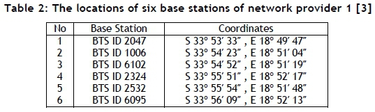
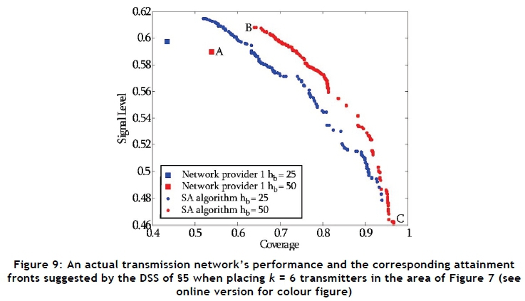
Under the assumption that all antennae are located at a height of h_b= 25 m above ground level, it was found that the transmitter locations in Table 2 achieve a coverage value of C(x) = 0.4356 and an average signal level of S(x) = 0.5976. When the assumed base station antennae heights are increased to h_b= 50 m, however, the values C(x) = 0.5409 and S(x) = 0.5897 are obtained. These values are plotted in Figure 9, together with the associated attainment fronts returned by the DSS for the placement of k = 6 transmitters.

It is acknowledged that the performance measure values reported above only incorporate coverage provided by those transmitters actually located within the specific area considered in this case study. As a result, there may be areas, especially along the periphery of the study area shown in Figure 7, that receive coverage from base stations located outside the area considered for transmitter placement in this case study.

Assuming base station antennae heights of h = 50 m above ground level, the view shed plot and signal level heat map of the existing transmitter network, corresponding to the point A in Figure 9, are shown in Figures 10 (a) and (b) respectively.

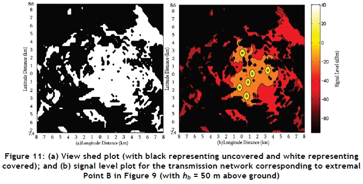
The view shed plots and signal level heat maps for the transmitter placements corresponding to the extremal points B and C in Figure 9 are similarly shown in Figures 11 and 12 respectively. The transmitter configuration corresponding to the extremal point denoted by B in Figure 9 is seen to outperform the existing network in both the coverage and the average signal level objectives, attaining performance values of ( ) = 0.6408 and ( ) = 0.6079.

The transmitter configuration corresponding to the extremal point C in Figure 9 outperforms the existing transmitter configuration in the coverage objective, attaining a value of ( ) = 0.9665. The existing network outperforms this configuration, however, in terms of the average signal level objective, for which a value of ( ) = 0.4614 is achieved.

 

7 CONCLUSION AND FURTHER WORK

Although still widely-used and widely-applicable (especially in the Southern African context), it is acknowledged that 2G mobile telecommunication network technology, which was the focus of this paper, is dated and so will be phased out over time. This technology, however, still forms the basis of most of the mobile networks currently in operation, and its infrastructure is used almost exclusively for voice traffic, keeping the 3G and 4G channels open for the improved download speeds achievable by 3G and 4G technology. Due to the increased range of 2G network technology over 3G and 4G network technology, the former networks are widely used in rural areas where large areas need to be covered. In these areas, the demand for high download speeds is typically not as large as in urban centres. This may be attributed to the lower income households typically associated with rural areas in Southern Africa, resulting in the use of more basic feature phones instead of the more costly data-intensive smartphones.

During the course of the literature survey that was performed as part of the preparation for this paper, we could find no case of the transmitter facility location in which a truly multi-objective optimisation approach was adopted. In the case of Mathar and Niessen [16], for example, a weighted objective function was used instead, while Krzanowski and Raper [14] implemented a convex combination of objective functions in their solution approach. Since the objective functions involved in radio transmitter placement problems typically differ in units, and their values are thus difficult to compare directly (even when normalised), it was decided rather to adopt a bi-objective modelling approach in this paper. This seems to be a novel approach in the context of 2G transmitter placement decisions.

The dominance-based multi-objective SA algorithm is well suited to solving the transmitter facility location problem considered in this paper, as indicated by the quality of the solutions uncovered in the case study in §6. In this case study, transmitter configurations were uncovered by the SA algorithm that outperform the existing network of network provider 1 by a significant margin in terms of both the coverage and the average signal level objectives.

Since time is typically not a critical factor during the mobile telecommunication network planning phase, exact solution approaches - which may take considerably longer than the method of SA to converge to feasible solutions - can be investigated. As an alternative approximate solution approach, a comparison between the single-threaded SA algorithm implemented in this paper and multi-threaded alternatives (such as a genetic algorithm or a particle swarm optimisation algorithm) can also be conducted to determine which algorithm yields the best trade-off between solution quality and computation time.

The DSS developed in this paper can be further validated by applying it to other case studies incorporating different terrain elevation data to test its flexibility in different contexts. In order to improve on the current DSS, post-optimisation decision support can also be included to facilitate a choice of one of the solutions forming part of the non-dominated front for implementation. A further improvement that may be incorporated into the current DSS is to develop the functionality required to be able to enter a set of transmitter locations that have already been placed, and then to use the DSS to add transmitters to the network, in addition to the existing transmitter locations, in pursuit of the coverage and average signal level maximisation objectives.

Finally, due to the multipath nature of radio wave propagation, interference in wireless environments between orthogonal signals can never be completely avoided. Amaldi et al. [1] define one measure of signal interference, called the signal interference ratio (SIR), as

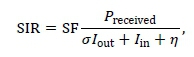
where P_recievedis the received signal strength at the demand point, σis an orthogonality loss factor, I_inis the total interference caused by signals transmitted from the same base station (called inter-cell interference), I_outrepresents the interference resulting from signals transmitted from other base stations (called intra-cell interference), r is the thermal noise power, and SF is a spreading factor - defined as the ratio between the spread signal rate and the user rate. This latter factor essentially takes the locations of different users with respect to one another into account when determining the level of interference experienced. Ideally, the SIR should be kept as low as possible to improve the quality of service. Incorporating the minimisation of the SIR as a third placement objective in the DSS of §5 might be a desirable extension to the work in this paper.

 

REFERENCES

[1] Amaldi, E., Capone, A., Malucelli, F. & Mannino, C. 2006. Optimization problems and models for planning cellular networks, pp. 917-939 in Resende, M. & Pardalos, P.M. (eds), Handbook of optimization in telecommunications, Springer, New York.         [ Links ]

[2] Busetti, F. 2003. Simulated annealing overview. Online reference available at: http://www.cs.ubbcluj.ro/-csatol/mestint/pdfs/Busetti_AnnealingIntro.pdf        [ Links ]

[3] CellMapper.net2015. CellMapper, Online reference available from https://www.cellmapper.net/map        [ Links ]

[4] Costa, A.M. 2005. A survey on Benders decomposition applied to fixed-charge network design problems, Computers and Operations Research, 32(6), pp. 1429-1450.         [ Links ]

[5] Daskin, M.S. 1995. Network and discrete location models, algorithms and applications, John Wiley & Sons, New York.         [ Links ]

[6] Dreo, J., Petrowski, A., Siarry, P. & Taillard, E. 2006. Metaheuristics for hard optimization: Methods and case studies, Springer, Berlin.         [ Links ]

[7] Feuerstein, M.J., Blackard, K.L., Rappaport, T.S., Seidel, S.Y. & Xia, H.H. 1994. Path loss, delay spread and outage models as functions of antenna height for microcellular system design, IEEE Transactions on Vehicular Technology, 43(3), pp. 487-498.         [ Links ]

[8] Fleury, B.H. & Leuthold, P.E. 1996. Radiowave propagation in mobile communications: An overview of European research, IEEE Communications Magazine, 34(2), pp. 70-81.         [ Links ]

[9] Groupe Speciale Mobile Association. 2014. The mobile economy: sub-Saharan Africa. (Unpublished) Technical Report.         [ Links ]

[10] Hata, M. 1980. Empirical formula for propagation loss in land mobile radio services, IEEE Transactions on Vehicular Technology, 29(3), pp. 317-325.         [ Links ]

[11] Hristov, H.D. 2000. Fresnel zones in wireless links, zone plate lenses and antennas, Altech House Inc., Norwood.         [ Links ]

[12] Iskander, M.F. & Yun, Z. 2002. Propagation prediction models for wireless communication systems, IEEE Transactions on Microwave Theory and Techniques, 50(3), pp. 662-673.         [ Links ]

[13] Kirkpatrick, S., Gelatt, C.D. & Vecchi, M.P. 1983. Optimization by simulated annealing, Science, 220(4598), pp. 671-680.         [ Links ]

[14] Krzanowski, R. & Raper, J. 1999. Hybrid genetic algorithm for transmitter location in wireless networks, Computers, Environment and Urban Systems, 23(5), pp. 359-382.         [ Links ]

[15] Kürner, T. 1999. COST Action 231 digital mobile radio towards future generation systems, (Unpublished) Technical Report, European Cooperation in the Field of Scientific and Technical Research.         [ Links ]

[16] Mathar, R. & Niessen, T. 2000. Optimum positioning of base stations for cellular radio networks, Wireless Networks, 6(6), pp. 421-428.         [ Links ]

[17] McKinney, A.L. & Agarwal, K.K. 1992. Development of the Bresenham line algorithm for a first course in computer science, The Journal of Computing Sciences in Colleges, 8, pp. 70-81.         [ Links ]

[18] OpenTopography.org2015. OpenTopograghy: A portal to high-resolution topography data and tools, [Online] [Cited October 2nd, 2015]. Available from http://opentopo:sdsc:edu/gridsphere/gridsphere?cid=datasets        [ Links ]

[19] Reed, M., Jotishky, N., Newman, M., Mbongue, T. & Escofet, G. 2013. Africa telecoms outlook 2014: Maximising digital service opportunities, (Unpublished) Technical Report, Informa.         [ Links ]

[20] Seidel, S.Y. & Rappaport, T.S. 1994. Site-specific propagation prediction for wireless in-building personal communication system design, IEEE Transactions on Vehicular Technology, 43(4), pp. 879-891.         [ Links ]

[21] Sherali, H.D., Pendyala, C.M. & Rappaport, T.S. 1996. Optimal location of transmitters for micro-cellular radio communication system design, IEEE Journal on Selected Areas in Communications, 14(4), pp. 662-673.         [ Links ]

[22] Smith, K., Everson, R.M. & Fieldsend, J.E. 2004. Dominance measures for multi-objective simulated annealing, Proceedings of the 2004 Congress on Evolutionary Computation, pp. 23-30.         [ Links ]

[23] Smith, K., Everson, R.M., Fieldsend, J.E., Murphy, C. & Misra, R. 2008. Dominance- based multiobjective simulated annealing, IEEE Transactions on Evolutionary Computation, 12(3), pp. 323-342.         [ Links ]

[24] Socioeconomic Data and Applications Center (SEDAC). 2015. Gridded population of the world (GPW), [Online] [Cited October 2nd, 2015]. Available from http://sedac:ciesin:columbia:edu/data/set/gpw-v3-population-count.         [ Links ]

[25] Triki, E., Collette, Y. & Siarry, P. 2005. A theoretical study on the behaviour of simulated annealing leading to a new cooling schedule, European Journal of Operational Research, 166, pp. 77-92.         [ Links ]

[26] Tutschku, K. 1998. Demand-based radio network planning of cellular mobile communication systems, Proceedings of the 17^th Annual Joint Conference of the IEEE Computer and Communications Societies, pp. 1054-1061.         [ Links ]

[27] Tutschku, K. & Tran-Gia, P. 1998. Spatial traffic estimation and characterization for mobile communication network design, IEEE Journal on Selected Areas in Communications, 16(5), pp. 804-811.         [ Links ]

[28] Weisman, C.J. 2002. The essential guide to RF and wireless, 2^nd ed., Pearson Education, Upper Saddle River.         [ Links ]

[29] Winston, W.L. 2004. Operations research: Applications and algorithms, 4^th ed., Brooks/Cole, Belmont.         [ Links ]

 

 

Submitted by authors 15 Feb 2016
Accepted for publication 5 Apr 2016
Available online 12 Aug 2016

 

 

# Author was enrolled for an MEng (Industrial) degree in the Department of Industrial Engineering, Stellenbosch University, South Africa
* Corresponding author vuuren@sun.ac.za