GENERAL ARTICLES

 

Exploiting deterministic maintenance opportunity windows created by conservative engineering design rules that result in free time locked into large high-speed coupled production lines with finite buffers

 

 

C. Durandt^{I, #, *}; E.v.d.M. Smit^I; N.D. du Preez^II

^IUniversity of Stellenbosch Business School, South Africa
^IIDepartment of Industrial Engineering, Stellenbosch University, South Africa

 

 

---

ABSTRACT

Conservative engineering design rules for large serial coupled production processes result in machines having locked-in free time (also called 'critical downtime' or 'maintenance opportunity windows'), which cause idle time if not used. Operators are not able to assess a large production process holistically, and so may not be aware that they form the current bottleneck - or that they have free time available due to interruptions elsewhere. A real-time method is developed to accurately calculate and display free time in location and magnitude, and efficiency improvements are demonstrated in large-scale production runs.

---

OPSOMMING

Konserwatiewe ingenieursontwerpreëls vir groot reeksgekoppelde produksieprosesse lei tot beskikbare vrye tyd (ook bekend as 'kritieke dooie tyd' of 'onderhoudsgeleenthede'), wat indien nie gebruik word nie, onbenutte tyd tot gevolg kan hê. Operateurs is nie in staat om 'n grootskaalse produksieproses op holistiese wyse te beoordeel nie, en mag gevolglik nie besef dat hulle op 'n bepaalde stadium óf die knelpunt is óf dat daar vrye tyd beskikbaar is as gevolg van onderbrekings elders nie. 'n Intydse metode is ontwikkel om vrye tyd akkuraat te bereken en te vertoon, beide wat posisie en grootte betref. Effektiwiteitsverbeterings word aangetoon in grootskaalse produksielopies.

---

 

 

1 INTRODUCTION

Coupled production lines face seemingly unpredictable idleness at workstations, caused by the stochastic behaviour of breakdowns and the propagation of these stoppages up and down the coupled manufacturing line. Common engineering design rules dictate that, to protect one key quality production process, up- and downstream machines should have a higher throughput and should be connected via a very large but finite buffer, sized to allow the key machine to run without interruption. These design rules are often overstated, and result in excessive idleness in upstream and downstream machines. This paper describes a method that shows how excessive free time at each production machine is calculated accurately and is displayed in location and magnitude. An experiment carried out at the Valpré water bottling plant in Heidelberg, South Africa is used to describe the improvement in efficiency that can typically be obtained by training the operators in this new method.

1.1 Background

The concept of 'free time' was contemplated from observations of a large coupled beer manufacturing production line in Durban, South Africa in 1998. The observations were part of a project to identify how the machine operators could benefit from the introduction of innovations in information technology in the workplace. Initially, the focus was on quality and the recording of quality data by production operators. It was from observations of operator behaviour that long periods of seemingly unpredictable idleness became evident.

Production engineers use a design rule, commonly known as the 'V-profile', in specifying equipment in the fast-moving consumer goods and similar high-speed packaging industry. The first author defined the over-design of this V-profile, resulting in the creation of free time, in 1998.

1.2 Assumptions and abbreviations

This paper describes a technique to calculate free time deterministically. The technique works for coupled production processes with finite inter-stage buffers where the V-profile design rule has been applied. Typical simplifying assumptions used in theoretical research (such as random failures are normally distributed; machine throughput speeds are constant; and buffer capacities are equal) do not need to apply when using this technique. Thus this technique can be applied in many real-life coupled production processes without limiting assumptions.

The following variables and their abbreviations are introduced:

A = Accumulator

AL = Accumulator level

CCM = Current constraint machine

CD = Countdown

CQ = Clear quantity

DFT = Dynamic free time

FT = Free time

HTR = Historic throughput rate

M = Machine

MATT = Minimum accumulator travel time

MOW = Maintenance opportunity windows

PDT = Prime delay time

PQ = Prime quantity

RTR = Relevant throughput rate

SFT = Static free time, also known as breakdown free time (BDFT).

1.3 Free time and maintenance opportunity windows

Free time is the time available for production machine operators to stop their machine due to inherent spare capacity, or due to the propagation of the effect of a stoppage elsewhere on the production line.

A machine can be stopped to use free time without affecting the overall performance of a coupled manufacturing production process. Free time is different from idle time, as idle time is imposed on a machine by blocking or starvation. Free time is the real-time calculation of future inevitable idle time.

The concept of 'maintenance opportunity windows' (MOW) has been defined [1], and analytical algorithms and simulation-based calculations of MOWs have been provided by analysing the relationships between the number of buffer occupancies and cycle times in small buffer systems. However, all the previous MOW models that have been analytically developed [1, 2, 3, 4] can only deal with deterministic systems. For example, cycle times are assumed to be constant and fixed, and there are no random downtimes in the system. In fact, when implemented in practice, the production line was seen to become fragile to the unexpected random downtimes that followed when maintenance had been conducted for a deterministic MOW duration in actual production lines. This is because buffers in transfer lines are almost depleted, and any stoppages before the line recovers its nominal capacity will jeopardise the intended favourable flow of production. To overcome such uncertainties and high risks, earlier researchers [1, 3] have suggested using simulation models that can handle uncertainties to calculate MOWs.

 

2 DYNAMIC OR TRANSIENT FREE TIME

The word 'dynamic' in this context refers to change over time. The constraint is moving around the production process; it does not always remain where it was designed to be. Dynamic free time (DFT) is the free time a machine has, due to the levels in the accumulators and throughput of the other machines in the production process. A machine can gain DFT if it is performing faster than its calculated steady state, and it can lose DFT if it is underperforming. Variance in the performance of specific machines will induce the dynamic characteristic of free time.

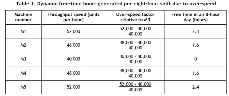
DFT is available at machines that have higher speeds than the key (bottleneck) machine. DFT increases when machines feeding - or those drawing from - the drum (bottleneck) machine have run faster than the drum machine for some period, and starvation or blocking is about to occur. Faster machines have to wait for slower machines because they are connected in a coupled manufacturing system with finite buffers. Table 1 below shows a five-machine model where throughput speeds were assigned, and the over-speed factor was calculated; the last column shows the total DFT per machine in an eight-hour shift.

 

Table 1 - Click to enlarge

 

In Figure 1 we plotted the throughput rates on the Y-axis and the machines on the X-axis. The DFT presented is the area under the V-profile. Each machine has free time that is independent of the others. Four different operators can use these times concurrently.

 

 

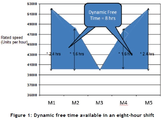
We can thus add the total DFT for an eight-hour shift as follows:

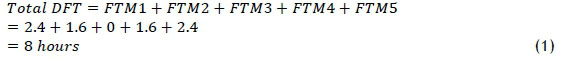
These results show there are eight hours of free time that can be used by the operators of M₁, M₂, M4, and M5 during a shift if the key machine runs at 100 per cent efficiency.

 

3 STATIC FREE TIME

Static free time (SFT), also known as 'breakdown free time' (BDFT), is the free time that all the other machines get when the bottleneck machine is stopped or breaks down. The concept of free time relies here on human intervention to obtain the maximum benefit. An operator would estimate the downtime at the bottleneck machine when the machine breaks down. It is therefore important that operators are trained in the technique of conservatively estimating anticipated downtime. This downtime information is then shared live - via a wireless link, in the case of the Valpré experiment detailed later in the paper - with all the other operators in the coupled process. The other operators can then use the BDFT to perform opportunistic preventative maintenance.

BDFT normally becomes available from unreliability at M₃ (the bottleneck). The bottleneck is usually at the key machine, but any other machine can become the bottleneck if it becomes more unreliable than the key machine, and can sporadically become the source of BDFT.

In Figure 2, the key machine M₃ experienced a combined total of one-hour stoppages during the eight-hour shift. This equates to achieving 87.5 per cent final efficiency for the shift. The total free time available at all the other machines due to the one-hour stoppage at the key machine M₃ equates to five hours of BDFT. The total free time for the two types of free time for this example is the sum of the DFT and the BDFT.

 

 

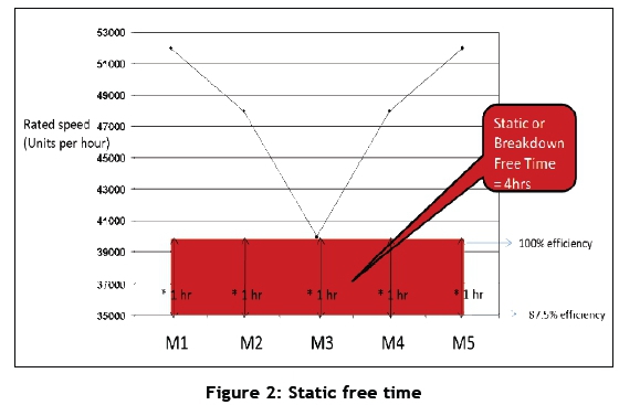
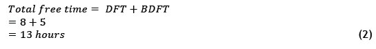
The total free time resulting from DFT and BDFT is 13 hours of free time during an eight-hour shift.

 

4 DETAILED DESCRIPTION OF THE METHOD

A coupled production process (Figure 3 below) is modelled as a set of pumps in series, with liquid tanks between them to represent the accumulators typical of finite buffer production processes.

 

Figure 3 - Click to enlarge

 

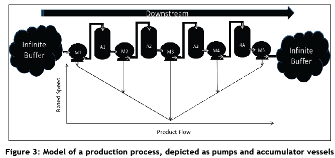
In this model, pumps M₁ to M₅represent five production machines, and buffer tanks A1 to A4 represent four accumulators between the production machines. For this model, we assume that there is infinite buffer storage before M1 and after M5. The fastest machines are M1 and M5; the slowest machine is M3.

4.1 The machine matrix

The machine matrix is developed for the general case for free-time calculations. The matrix in Figure 4 plots the various machine types and the number of machines of each type. There are i types of machine positions and j machines in each machine position.

 

 

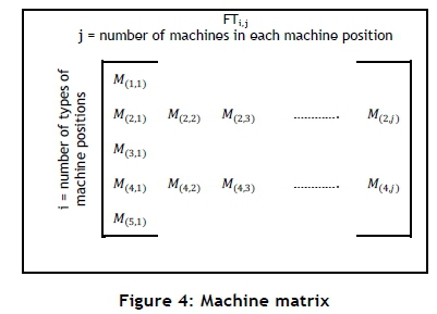
For the types of machine positions, (i) is defined as follows:

• Type-1 = Start machine with infinite buffer on its in-feed and finite buffer on its discharge.

• Type-2 = A machine with a finite buffer on either side; its in-feed machine is faster and its discharge machine is slower.

• Type-3 = The bottleneck or key machine, with finite buffers on both sides; its in-feed and discharge machines are faster.

• Type-4 = A machine with a finite buffer on either side; its in-feed machine is slower and its discharge machine is faster.

• Type-5 = End machine with infinite buffer on its discharge, and an infinite buffer on its in-feed.

We therefore have i = 1, 2, 3, 4, and 5.

For each machine position type (i), there are the following numbers of machines (j):

• One type-1 machine;

• Any number of type-2 machines;

• One type-3 machine;

• Any number of type-4 machines; and

• One type-5 machine.

Therefore j = 1, for type-1 machines.

We therefore have:

j = 1, for type-1 machines

j = 1, 2, 3, 4.......∞ for type-2 machines

j = 1, for type-3 machines

j = 1, 2, 3, 4.......∞ for type-4 machines

j = 1, for type-5 machines

4.2 The accumulator matrix

The accumulator matrix is developed for the general case. The matrix in Figure 5 plots the accumulator types and the number of accumulators for each type. There are i types of accumulator positions and j accumulators in each accumulator position.

 

 

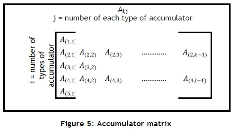
There are five types of accumulator position, defined as follows:

• Type-1 is the first machine's accumulator, and is defined as the accumulator following the first machine.

• Type-2 is defined as the accumulator(s) following a type-2 machine but not connecting to the bottleneck machine.

• Type-3 are the accumulators preceding and following the bottleneck machine.

• Type-4 is the accumulator(s) following the type-4 machine and not connecting to the type-5 machine.

• Type-5 is defined as the accumulator following a type-4 machine and connecting to the type-5 machine. It is also the last accumulator on the production line.

We therefore have i = 1, 2, 3, 4, and 5.

For the j accumulator types, we have the following number of accumulators per type:

• One type-1 machine's accumulator;

• Any number of type-2 machines' accumulators;

• Two type-3 machines' accumulators;

• Any number of type-4 machines' accumulators; and

• One type-5 machine's accumulator.

We therefore have:

j = 1, for a type-1 accumulator

j = 1, 2, 3, 4.......∞ for type-2 accumulators

j = 2, for type-3 accumulators

j = 1, 2, 3, 4.......∞ for type-4 accumulators

j = 1, for type-5 accumulators.

 

5 SLEEP FREE TIME - STATIONARY

Sleep free-time equations calculate free time during the inactive state of a production process. During this stationary state, the free-time calculations are stationary, in contrast with the transient state of the start-up, normal running, blocking, starvation, and run-out calculations. Sleep free time is, for example, the minimum time that a maintenance worker can claim the production machine when the production process is not active. The production process can start at any moment, but the product needs to travel through the accumulators to reach all the production machines down the line. The total sum of the time it takes to reach the relevant machines down the line and prime its preceding accumulators is the sleep free time.

5.1 Sleep free-time calculations for all machine types

5.1.1Machine type: i = 1

During the sleep state, the free time on the first machine M₁ (i = 1 and j = 1) is zero, as the machine can be required to start work at any time. The first machine M₁, in a coupled manufacturing process, borders an infinite buffer at its in-feed side and a finite buffer on its discharge side. The expected arrival time of the product at the in-feed of the first machine cannot be determined accurately using the free-time model. We therefore have to assume that the product can arrive at any time at M1, and the sleep free time is therefore zero.

It therefore follows that, for sleep free time for M(1,1):

5.1.2Machine type: i = 2

The sleep free time of the second machine M₂ in a production process is expressed as FT_m(2,1), and is bordered by empty finite buffers in the sleep state. The free time at the second machine-station FT_m(2,1) is the sum of the minimum accumulator travel time (MATT) for A_(1,1), and the prime delay time (PDT) (the time it will take to prime A_(1,1)).

It therefore follows that for the second machine in the model:

The prime quantity (PQ) is the level that is required in an accumulator, preceding the machine that draws from the accumulator, for the machine to start. 'Required level' means the extent to which the buffer must be filled for the machine to start working productively. This level should be sufficient for the machine to start and run continuously for a productive period. The productive period is a function of the type of operation, as some machines must run continuously for days, and others for a few seconds, to be seen as productive.

In the two examples of the buffer tank with pumps on both sides in Figure 6, the level in the tank is primed only when the prime quantity level is reached. In the first image in Figure 6, the buffer is empty and the discharge pump cannot start. The fill level needs to be high enough to allow the pump to start without cavitation. Given the V-profile design rule, the pump on the in-feed side of the buffer illustrated in Figure 6 will have a higher throughput. This will cause the level to rise until the accumulator is full and the upstream machine becomes idle.

 

 

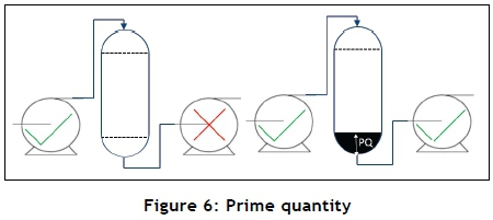
The prime quantity is a constant, but could vary slightly over time as process conditions change. The quantity is ultimately a function of the rate at which the accumulator can be primed and, due to the stochastic nature of the production machine performance, this is not constant. Historical throughput rate (HTR) is used in the case of sleep free time because the line is not running, and real-time throughputs are not available in the current data.

The minimum time it takes to prime accumulator A_(1,1), the prime delay time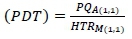

Therefore:

For the general solution, k number of type-2 machines can be present.

Sleep free time is therefore the sum of the type-1 sleep free time plus all the preceding type-2 machines, and is expressed as:

5.1.3 Machine type: i = 3

During the sleep state, the free time on the bottleneck machine M3 is the sum of the minimum accumulator travel time (MATT) for all the preceding accumulators, the prime delay time (PDT) of all the preceding accumulators, and the time it takes to fill the accumulator after the bottleneck machine to its clear quantity (CQ).

CQ is the level in an accumulator, once the accumulator has drained sufficiently, for the upstream machine to start and run for a productive period. In the first picture in Figure 7 below, the full accumulator prevents the pump from starting; in the second depiction, the pump can start and run productively - especially in this case, where the downstream machine has a higher throughput rate than the upstream machine. The accumulator level will drop, and eventually the downstream machine will become idle.

 

 

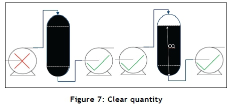
The clear quantity is a constant, but could also vary slightly over time as the process conditions change. The quantity is ultimately a function of the rate at which the accumulator can be cleared and, due to the stochastic nature of production machine performance, this is not constant.

The minimum time it could take to fill the accumulator after the bottleneck machine to its clear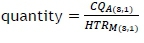

It therefore follows that sleep free time for the bottleneck machine can be calculated as follows:

5.1.4 Machine type: i = 4

The sleep free time for machines following the bottleneck machine M4 is the sum of the sleep free time at the bottleneck machine FT_M(_3,1) and all the type-4 sleep free times before the specific type-4 machine being expressed.

It therefore follows that, for type-4 machines, sleep free time with k number of type-4 machines can be expressed as:

5.1.5 Machine type: i = 5

The sleep free time for the last machine in the process, M₅, is the sum of the sleep free time at the last type-2 machine, the minimum time it takes to travel through the last finite buffer of the process A(5,1), and the time it takes to fill the final buffer A(5,1) to its prime quantity.

It therefore follows that, for the type-5 machine, the sleep free time can be expressed as:

5.2 The current constraint machine during the sleep state

In order to add breakdown free time, the current constraint machine must always be identified. Each process state has a different current constraint machine (CCM) rule. During the sleep process state, the CCM is always the first machine in the process M(1, 1), bounded by the infinite buffer on its in-feed and the finite buffer on its discharge.

From the sleep state, the production process enters the start-up mode. A countdown (CD) starts on each machine, starting with the sleep free time total and counting down to zero. The 'handover' from sleep free time to normal running is done with the countdown. The inclusion of the countdown in the calculation of normal running free time is included in Section 6.1.2 of this paper.

 

6 START-UP AND NORMAL RUNNING FREE TIME - TRANSIENT

During the transient state, free time is calculated by dividing the accumulator quantity by the live throughput rate of the machine filling or draining the accumulator (whichever is relevant, given the prime or clear condition):

When the first production machine starts running, the transient state is triggered, and each machine starts a countdown from the stationary state free time to zero. This countdown (CD) is used in all the equations during the start-up state. Start-up and normal running formulations are combined by a formula that returns the maximum of the various building blocks for accumulators in the free-time concept. For example:

will return the biggest number between X and Y.

In this way, start-up and normal running can also be handled in the same equation.

6.1 Start-up and normal running free-time calculations

Four generic types of free time are defined as follows:

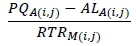
Type-1: The time to fill an accumulator upstream from the key machine to its prime level is:

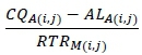
Type-2: The time to fill an accumulator downstream from the key machine to its clear level is:

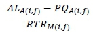
Type-3: The time to drain an accumulator upstream from the key machine to its prime level is:

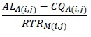
Type-4: The time to drain an accumulator downstream from the key machine to its clear level is:

The four generic types of DFT are developed into 16 building blocks to construct the available free time for any number of production machines.

A summary of the sixteen building blocks is set out in Table 2 below.

 

Table 2 - Click to enlarge

 

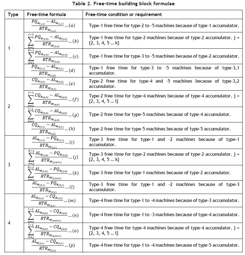
6.1.1 Machine type: i = 1

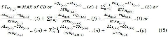
For a five-machine solution, during start-up and normal running the free time at the first machine M₁ is the largest of the time available to bring accumulators 1,1 and 3,1 to their prime quantity level OR, the free time available in accumulators 3,2 and 5,1 in bringing them down to their clear quantity:

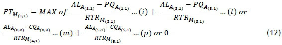
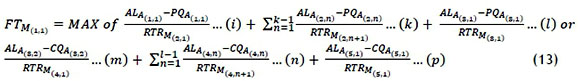
The general solution for k number of type-2 machines and l number of type-4 machines is:

Note: There is no countdown for machine type: i = 1, because its sleep free time is always zero.

6.1.2Machine type: i = 2

For a five-machine solution, during start-up and normal running, the free time at the type-2 machine FTM2 is the largest of the following four numbers:

1. The countdown CD of the particular machine;

2. The time it takes to bring accumulator 1 up to its prime level;

3. The time it takes to bring accumulator 3,1 down to its prime level; or

4. The time it takes to bring accumulators 3,2 and 5 down to their clear quantity.

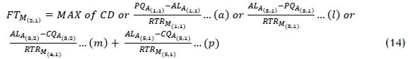
The solution for k number of type-2 machines and l number of type-4 machines is:

6.1.3Machine type: i = 3

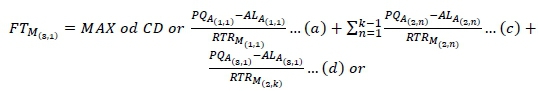
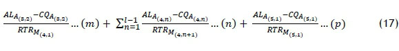
For a five-machine solution, during start-up and normal running, the free time at the type-3 machine FTM3 is the largest of the following three numbers:

1. The countdown of the type-3 machine;

2. The time it takes to bring accumulators 1,1 and 3,1 from below their prime quantity back to their prime level;

3. The time it takes to bring the current level of accumulators 3,2 and 5,1 down to their clear quantity.

The solution for k number of type-2 machines and l number of type-4 machines is:

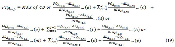
6.1.4Machine type: i = 4

For a five-machine solution, during start-up and normal running, the free time at the first type-4 machine FTM1 is the largest of the following four numbers:

1. The countdown CD of the particular machine;

2. The time it takes to bring accumulators 1 and 3,1 up to prime level;

3. The time it takes to bring accumulator 3,2 up to its clear level; or

4. The time it takes to bring accumulator 5 down to its clear level.

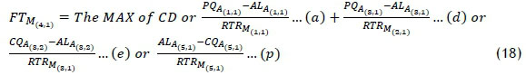
The solution for k number of type-2 machines and l number of type-4 machines is:

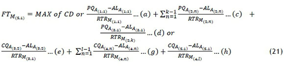
6.1.5Machine type: i = 5

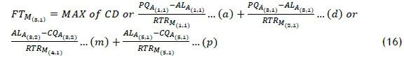
For a five-machine solution, during start-up and normal running, the free time at the type-5 machine FTM5 is the largest of the following three numbers:

1. The countdown CD of the particular machine;

2. The time it takes to bring accumulators 1 and 3,1 up to prime level; or

3. The time it takes to bring accumulators 3,2 and 5 down to clear level.

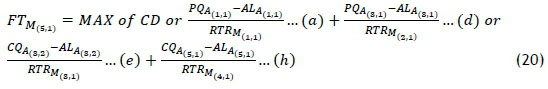
The solution for k number of type-2 machines and l number of type-4 machines is:

 

7 THE EXPERIMENT

An experiment was conducted at the Valpré water bottling facility, owned by Coca-Cola, in Heidelberg, South Africa to test the efficacy of the model. Specific free-time formulae were derived for the general free-time calculations developed in the section above. Hardware was designed and built to deal with the large flow of signals and data in the wireless network. Computer code was programmed to run the required algorithms for the free-time calculations. Operators were trained in the use of the free-time system and in the concept of the productive use of free-time during MOWs. Three propositions were tested.

7.1 Proposition 1: Demonstrate that free time can be calculated accurately in real-time

To test this proposition, the acid test was formulated. The acid test is defined as a physical test performed by stopping a production machine during the normal course of its duties for a period - no longer than the free time - and starting the machine again before the free time runs out. The test then continues by observing the effect the stoppage has had on the current bottleneck machine. A successful acid test is one where the test stoppage did not influence the bottleneck machine.

7.2 Proposition 2: Demonstrate that operators can start production processes better, given free-time start-up information

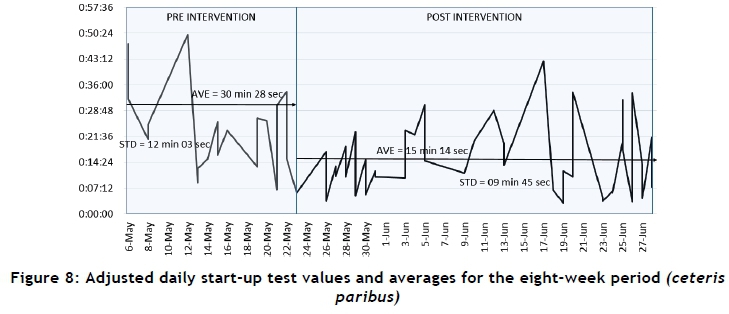
To test this proposition, the start-up test was formulated. A start-up test is performed during the start-up of a production process by measuring the time (duration) between the theoretical ideal start-up moment (calculated by the free-time formulae) and the actual start-up moment (performed by the operator and observed by the tester).

7.3 Proposition 3: Demonstrate that operators can stop production processes judiciously, given accurate free-time information

To test this proposition, the judicious use test was formulated. This test is performed during the normal running of the production process to evaluate whether the operator has used free-time information to execute discretionary stoppages judiciously - stopping the production machine at just the right times.

 

8 TEST RESULTS

The three propositions were tested continually over a period of eight weeks. The test period was from 6 May to the end of June 2014. No samples were taken during this time, as the data collected represented the full population of available data.

8.1 The acid test

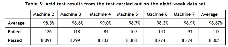
The percentage of successful acid tests was calculated using an algorithm that identifies acid test events, and does this independently of operator input or awareness. During the experiment, a total of 8,417 automated acid tests were conducted. Of these tests, 8,305 passed and 112 failed - a pass rate of 98.67 per cent (see Table 3).

These results proved that the free time calculated by the formulae was sufficiently accurate. The clear quantity could have been adjusted to increase the accuracy of the results further, but would only have led to free-time reduction.

8.2 The start-up test

In the experiment, the operator's start-up moment was matched to the theoretical best moment as calculated by the free-time system. The operators were trained and then presented with a freetime display. The experiment was repeated, but now the operators were requested to prepare their production machines in time to be ready for the indicated start-up moment. The difference between these two moments was plotted in Figure 8 over a period of eight weeks -i.e., three weeks before the intervention and five weeks thereafter. The average time difference improved from 30 minutes and 28 seconds to 15 minutes and 14 seconds. This represented an improvement of 15 minutes and 14 seconds. The standard deviation for this experiment was 12 minutes and 28 seconds before the operators were trained; this was reduced to 9 minutes and 45 seconds after the operators had been trained. Refer to Figure 8 below for a summary of the findings.

 

Figure 8- Click to enlarge

 

8.3 The judicious use test

The extent to which free time was used judiciously was recorded at machines 2, 3, and 4. The average free-time use efficiency was 80 per cent in the three weeks prior to the intervention. The free-time use efficiency increased by ten per cent to almost 90 per cent in the eight weeks after the intervention. This improvement clearly indicates the improved free-time use by production operators after the intervention. See the graph in Figure 9.

 

 

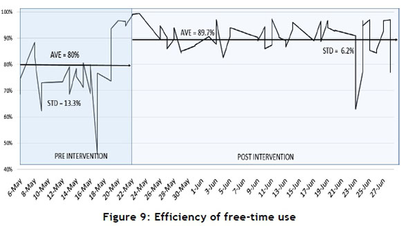
The standard deviation before the intervention was calculated at 13.3 per cent, and reduced to 6.2 per cent after the intervention. This shows that the variability in the results improved substantially.

This improvement in variability suggests a more controlled use of free time and fewer outliers. Operators have embraced the use of free time during normal operation.

The ultimate measure of improved performance on a production line is to produce more units in the same number of production hours. Overall line efficiency is the measure used for production performance. This measure also directly translates into financial value, and is calculated in the next section of this paper.

8.4 The results of overall production line efficiency

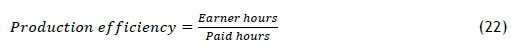
The overall efficiency of the production process was monitored throughout the experiment. The efficiency is calculated by dividing the earned hours by paid hours for each shift. The term 'earned hours' is the number of actual cases produced in the shift, divided by the throughput rate for the key machine. 'Paid hours' in the case of the Valpré plant are represented by an eight-hour shift.

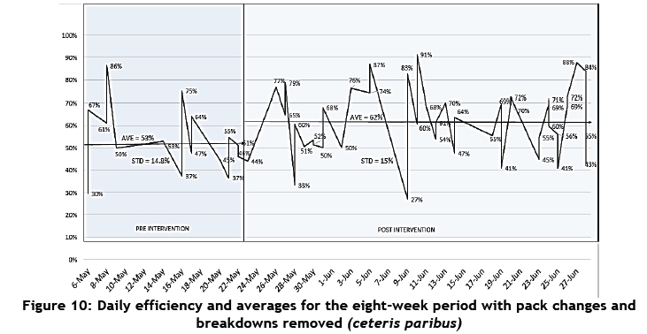
The average efficiency improvement was calculated at nine per cent, with the average efficiency before the intervention at 53 per cent and after the intervention at 62 per cent. The standard deviation improved from around 20 per cent prior to the removal of major breakdowns and pack changes to 15 per cent after the intervention. No improvement in the variation was observed from before the intervention to after the intervention. See Figure 10.

The financial value of a nine per cent production efficiency improvement can be expressed in hours saved per month to achieve the same production quantity. The plant normally operates six days per week and 16 hours per day. The plant therefore runs, on average, 25.2 days at 16 hours each, or 453.6 hours per month. The nine per cent saving on 453.6 hours result in a 40.8 hours saving per month. The shift labour running cost was calculated to be R 2,314.00 (South African Rand) per hour. The total saving per month therefore equates to R 94,466.70 (South African Rand).

 

9 CONCLUSION

The theory to calculate free time was tested for accuracy by using an acid test specifically designed for this purpose. Once an accurate free time had been presented to the operators, they were trained and requested to use the free time productively to improve the productivity on the production line. A test was developed to measure the extent to which the operators used the free time during startup and during normal running. A marked improvement in both these indicators was observed.

Finally, the overall performance of the production line was monitored, and a significant improvement in efficiency on the production line was observed. The Valpré experiment thus demonstrated that the productive use of free time or MOWs can result in improved production efficiency.

These results are significant in improving the productivity of the production lines of this type. Different configurations may be candidates for future research.

 

REFERENCES

[1] Chang, Q., Ni, J., Bandyopadhyay, P., Biller, S. & Xiao, G. 2007. Maintenance opportunity planning system, Journal of Manufacturing Science and Engineering, 129(3), pp 661-668.         [ Links ]

[2] Liu, J., Chang, Q., Biller, S. & Xiao, G. 2010. Transient analysis of downtimes and bottleneck dynamics in serial manufacturing systems, ASME Journal of Manufacturing Science and Engineering, 132(5), pp 1-9.         [ Links ]

[3] Gu, X., Lee, S., Liang, X., Garcellano, M., Diederichs, M. & Ni, J. 2013. Hidden maintenance opportunities in discrete and complex production lines, Expert Systems with Application, 40(11), pp 4353-4361.         [ Links ]

[4] Xia, T., Xi, L., Zhou, X. & Lee, J. 2012. Dynamic maintenance decision-making for series-parallel manufacturing system based on MAM-MTW methodology, European Journal of Operational Research, 221(1), pp 231-240.         [ Links ]

 

 

Submitted by authors 17 Sep 2015
Accepted for publication 28 Apr 2016
Available online 12 Aug 2016

 

 

# Author was enrolled for a PhD in the University of Stellenbosch Business School
* Corresponding author cdurandt@coca-cola.com