GENERAL ARTICLES

 

Mathematical and simulation techniques for modelling urban train networks

 

 

N. Wilson^{I, #}; C.J. Fourie^{I, *}; R. Delmistro^II

^IDepartment of Industrial Engineering Stellenbosch University, South Africa
^IIGroup Strategy Office PRASA, South Africa

 

 

---

ABSTRACT

Railway systems can pose complex problems for the scheduling and operation of trains. A passenger rail service's first priority is to provide a punctual and safe transport service to its customers. But doing so is a major challenge for rail network operators, as disruptions are inevitable, especially in densely-populated networks. Disruptions can be caused not only by infrastructure or rolling stock breakdowns, but also by maintenance activities, new rolling stock, or new train services. Managing these disruptions and predicting the extent of its effects is a crucial part of rail network operation. Mathematical models and simulation can be applied to these problems. This paper will review the literature concerning the modelling of train networks.

---

OPSOMMING

Spoorwegstelsels skep soms komplekse probleme met betrekking tot die skedulering en die bedryf van treine. 'n Passasiers-spoordiens se eerste prioriteit is om stiptelike en veilige vervoer te verskaf aan sy gebruikers. Om 'n stiptelike en betroubare diens te lewer is 'n groot uitdaging vir netwerk operateurs, aangesien trein dienste maklik ontwrig word in digbevolkte netwerke. Ontwrigtinge word nie net deur infrastruktuur en rollende materiaal falings veroorsaak nie, maar ook deur infrastruktuur onderhoud, nuwe rollende materiaal, en nuwe treindienste wat ingestel kan word. Die bestuur van dié ontwrigtinge en die akkurate vooruitskatting van die effek op die res van die netwerk is 'n kritiese komponent van die bedryf van 'n trein netwerk. Wiskundige modelle en simulasie metodes kan toegepas word op dié tipe probleme. Hierdie artikel bespreek die literatuur wat oor die modellering van trein netwerke handel.

---

 

 

1 INTRODUCTION

Railway network companies often need to model and simulate the operation of their trains. This need usually arises with the expansion or maintenance of infrastructure, or the addition of new rolling stock and services. Infrastructure expansion entails adding new links, stations, or additional lines on a specific route. Furthermore, perway, electrical, and signals maintenance all contributes to train operations being disrupted to some extent. And adding train services or new rolling stock requires major operations planning and rescheduling. Forecasting the effect on the operation of the network before the implementation of such changes is a crucial component of planning. Bottlenecks, line capacities, demand satisfaction, and delay propagations are all areas that need to be identified and calculated before large capital amounts are spent. This can be done through the use of mathematical models and simulation. The optimisation of existing operations can also be done using these tools.

 

2 OBJECTIVE

The objective of this paper is to review the literature on the different modelling techniques that are used to describe the operation of train networks. This will lay the groundwork for developing the most appropriate application of these techniques on whichever case study of train networks needs to be modelled by future research work. The two spectrums of modelling train networks, analytical models and simulation models, will be discussed. In section 2, mathematical models and heuristic algorithms will be discussed, while in section 3 simulation models will be covered.

2.1 Mathematical models and heuristics algorithms

Analytical models tend to be limited in scope and complexity, but they mostly form the basis on which simulation models are built. With the advances made in computer capabilities in the last 10 years, the use of analytical models has become scarce. Kozan and Higgens [1] developed an analytical model to estimate delays for individual trains and track links in an Australian rail network. They compared the results with those obtained from a simulation algorithm. For 93 per cent of the 157 scheduled trains, the analytical model's delay estimates were within 20 per cent of those of the simulation algorithm's estimates. This shows that if the scope of the model is small enough, analytical and simulation models can produce similar answers.

When it comes to optimising train schedules, heuristic algorithms are used, such as job shop, genetic, and Tabu-search algorithms. These heuristic algorithms will be discussed in later sections.

2.2 Queuing models

Queuing theory, which was originally referred to as 'telegraphic theory', was developed in the 1920s for telecommunication services. The application of this theory has since expanded to the computer, manufacturing, retail, services, and transport industries.

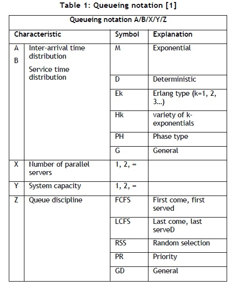
Queuing processes are usually described by six characteristics; these are listed by Gross et al. [2] as:

1. Arrival pattern of customers.

2. Service pattern of servers.

3. Number of service stages.

4. Number of service channels.

5. Queuing discipline.

6. Capacity of the system.

The arrival pattern in most queuing models is stochastic in nature, and follows a certain probability distribution of inter-arrival times. It can, however, also be deterministic, depending on the systems being modelled. When setting up the parameters for arrival, it is necessary to know if agents can arrive in bulk - i.e., simultaneously - and if so, the probability distribution of the size of the bulk. In some models, an agent can decide not to join the queue upon arrival; this is referred to as 'balked'. In some cases, an agent can enter a queue, and then lose patience after a while, and leave the queue; this is referred to as 'reneged'. Another case may be when there is more than one queue and an agent switches from one queue to another; this is called 'jockeying'. Further on, when an arrival distribution does not change over time, it is referred to as 'stationary'; and when it does change, it is called 'nonstationary'. Note that jockeyed and reneged arrivals are not considered in rail systems. Trains cannot arrive in bulk because of headway constraints forcing trains to have a certain time or distance buffer between them. Similarly, trains cannot renege or jockey in a queue (waiting track) if the driver becomes impatient. It is possible, however, for a train to balk. When a serious disruption occurs on a route, oncoming trains can be rerouted where possible, or even be cancelled.

Similar to arrival patterns, service patterns also have distributions describing the time an agent spends being serviced. Agents can also be serviced in bulk or individually. The service time can, however, be influenced by the size of the queue or arrival pattern. In such a case, it is referred to as a 'state-dependent service', but generally arrival and service patterns are assumed to be independent [1]. Another aspect of service time, as with arrival patterns, is that it may change over time - e.g., when learning takes place and the service process becomes quicker and more efficient. The same terms mentioned previously, 'stationary' and 'nonstationary', are used for such service processes. This is not usually applicable in rail systems, as trains have specified dwell times at stations.

How an agent is chosen for service from a queue is referred to as the queuing discipline. The most common discipline is the first-come-first-served (FCFS) principle; however, in some inventory systems, the last-in-first-out (LCFS) principle applies. Other systems have priority schemes that are usually called either 'pre-emptive' or 'non-pre-emptive'. Pre-emptive priority is when a high priority agent enters a queue, the service on a low priority agent is paused. and the high priority agent is serviced first. In the case of a non-pre-emptive priority, the high priority agent will be moved to the front of the queue, but will only be serviced when the agent being served at that moment is finished. Passenger rail systems mostly work on the FCFS principle, whereas freight rail systems might have different disciplines that take into account the importance of the freight content.

Some systems have limited queues, which creates a limited system capacity, such as a doctor's waiting room with a limited number of chairs. On the other hand, some queuing systems have infinite capacity, as in the case of judicial processes or waiting lists. In the case of rail systems where stations and sections are the servers, queues are limited.

Queuing systems can have more than one service channel. In general, it is preferred to have a single queue feeding multiple channels - e.g., customs at airports and railway stations with more than one platform. This usually applies in systems where the agents have no preference about which service channel they want to use. On the other hand, in systems like most supermarkets with multiple tills, customers line up in multiple queues.

The last aspect of queuing systems is stages of service. Systems may have more than one service stage; manufacturing systems are good examples of this. Parts will, for instance, be assembled and then moved forward to be checked for quality. If the quality is not satisfactory, the assembly will be fed back to the previous stage, or else the assembly will move forward to be painted. Passenger rail systems only have one service stage, while freight trains may have more (e.g., freight being unloaded and then the train moving to the hump yard).

The following points summarise queuing systems:

1. An agent arrives according to a certain probability distribution or fixed inter-arrival time.

2. The agent then enters or does not enter the queue, depending on the type of system.

3. The agent then moves from the queue to get serviced for a duration specified by the modeller. This can be for a stochastic or fixed time period.

4. After the agent is serviced, it leaves the system and the next agent in the queue is serviced, depending on the queuing discipline.

Huisman et al. [3] developed a queuing network model to compute the long-term performance of rail networks. To achieve this, a decomposition of the network and its detailed components was necessary. These components include stations, junctions, and sections. The network performance was measured by the mean delay and delay probability of the trains arriving at their destinations. Because train movements are not known over the long term, assumptions were made to simplify the modelling of stations. One of the assumptions is to model the storing tracks outside of the model. Thus, when a train finishes its route, it exits the model and is stored in a queue outside the model. The halting track is where the train starts its route and where the passengers alight or board the train. The next train can only enter the model after the train on the halting track has departed.

The occupation times at the halting tracks are assumed to be distributed exponentially and to be equal for all train types. The stations are modelled as multi-server queuing systems (since stations have more than one platform), with Poisson arrival distributions.

The same principles were applied to junctions and sections, except that these were single server queues. If a junction is occupied, the next train falls into the queue, until the junction is clear. This occupation time is also distributed exponentially.

Sections were broken up into signal blocks, with each block acting as a separate queuing system. Bottlenecks and delays were then calculated by adding up all the waiting times in the queues. These waiting times were compared with the practical delay times of the trains.

The model showed good accuracy, even though the timetable was not taken into account. Yuan and Hansen [4] and Meester and Muns [5] have both emphasised the lack of queuing models to consider timetables, since they are reliant on probability distributions for inter-arrival times. Moreover, fixed arrival and departure times were also not considered, and the impact of speed variations was neglected. Huisman et al. [3] instead suggested a way to capture speed variances among different train types by ignoring block (signalling) sections in a section between stations. However, the model does include one block section before and after each station, to ensure that trains do not arrive in bulk at stations. This means that, for instance, if a section has five signalling blocks, the middle three sections will be removed from the model and only the first and last sections will be included. This allows enough distance for a train with a different speed to have a significant variance in free running time; here, free running time refers to the time a train takes to travel between stations without any disruptions. The model of Huisman et al. [3] was applied to two major lines of the Dutch network, Rotterdam to Utrecht, and Den Haag to Utrecht. The traffic on this network is extremely heterogeneous, with three different train types (implying three different train speeds) running three different services.

 

 

De Kort et al. [6] also applied a similar queuing model, based on Wakob's approach, to Den Hague station in the Netherlands. Wakob's approach breaks up all the components of a station and analyses them independently as separate queues. Arrival and service times are both assumed to fit an Erlang distribution, resulting in Ει_<(λ)/Ε^μ)/1 queues for the whole queuing system. De Kort et al. [6] argued that service time variations should be dependent on running time and dwell time variations, instead of on independent probability distributions. It was found that this approach overestimates delays and, alternatively, models the 'worst case scenario'. This may be related to the fact that Wakob's approach returns the upper bound of the delay duration instead of the mean and standard deviation. Although this approach is inappropriate for delay propagation analysis, it can be useful for capacity planning purposes [6].

Queuing models can serve as a good alternative to simulation in order to estimate delays, although - as mentioned previously - modelling large networks becomes difficult to solve analytically. Kozan and Higgens [1] explain this complexity of train networks:

"A train network is complex in that it includes many intersections, uni- and bidirectional track links of various lengths, sidings, and track capacity. Train services vary with different upper velocities, slack time, scheduled stops, non-uniform departure times, and include train connections as described in the introduction of the paper. In the case of train connections and intersections, a train can suffer a delay from another that is scheduled much earlier and from a different part of the network."

"As well, the distribution of arrival times for each train at any station or intersection depends on the distribution of current delay, which can be different for each train service. Hence, delay to both the trains and at stations (or intersections) are interdependent. Therefore, the calculation of expected delay requires a solution of equations."

2.3 Job shop models

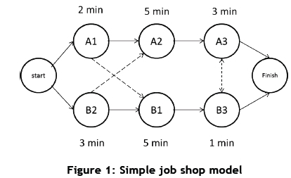
Branch and bound algorithms have been used to develop and optimise timetables. These models transform train networks into large job shop models. Typically, trains will be jobs and stations and sections will be machines. In job shop models, a number of different jobs need to be completed by a number of machines. A job will have a specified time and order that it has to spend at each machine. For example, Job A will use Machine 1 for two minutes, then Machine 2 for five minutes, and lastly Machine 3 for three minutes. Job B will first use Machine 2 for three minutes, then Machine 1 for five minutes, and end off with Machine 3 for one minute. Figure 1 shows an illustration of this simple model. It is important to note that each machine can only work on one job at a time. This means that when Job B is finished with Machine 2, Job A can move to Machine 2. Similarly, when Job A is finished with Machine 1, Job B can move to Machine 1. Whichever job finishes using Machines 1 and 2 first then moves to Machine 3. The other job will then have to wait for the first job to finish before moving to Machine 3. In the example illustrated in Figure 1, both jobs will arrive at Machine 3 at the same time. In such cases, priority rules can be implemented. Problems of this nature create the need to determine what the optimal sequence of machine use is; i.e., which job should use which machine when. Branch and bound algorithms are used to solve these problems. For further explanations of job shop models and branch and bound algorithms, refer to Gross et al. [2].

 

 

Rail networks can be similarly modelled, where trains are seen as jobs, and stations, sections, and junctions are seen as machines. There are, however, key differences between train network models and classical job shop models. These are listed as follows [7]:

• Jobs and machines do not have lengths as do trains and sections.

• While moving from one section to another, a train's 'head' will occupy the next section, while the 'tail' will occupy the current section. A train may thus occupy two sections at a time, whereas jobs can normally only occupy one machine.

• Train acceleration, deceleration, and cruising speed for a specific section cannot always be pre-defined, since it is dependent on the train in front.

• Trains can visit sections more than once, whereas jobs are mostly assumed to visit machines only once.

• Passing facilities such as passing loops on rail sections are equivalent to capacitated buffers or parallel machines. These are very difficult features to model with a standard job shop model.

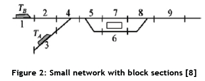
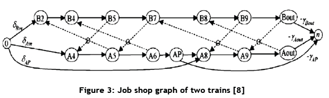
In Burdett and Kozan's [7] paper, the authors explain how these differences were incorporated in order to produce realistic results. D'Ariano et al. [8] developed a job shop model for the Dutch railway network. Figure 2 shows a small network on which the model in Figure 3 is based. Note that each block section is represented by a machine or a resource, as referred to in this paper, and Trains A and B are the jobs. A minimum headway of one signal block between trains is modelled and indicated by the dotted arrows in Figure 3. For example, Train A can only enter Block 5 when Train B has exited Block 7.

 

 

This model was expanded to model the Schiphol rail network, which includes the stations of Nieuw-Vennep, Hoofddorp, Amsterdam Lelylaan, and Amsterdam Zuid. The network consists of 86 block sections, 16 platforms, traffic in two directions, and 54 trains.

The model wished to solve the train scheduling problem for real-time rail network management. The objective function was to minimise the maximum secondary delays at all stations by all trains. It was found that these algorithms perform better than the despatching rules commonly used in relation to average and maximum delays.

Burdett and Kozan [9] used a hybrid job shop model with time window constraints to solve the train scheduling problem when adding additional train services. In their later work [7], they again used the job shop approach, but then further refined the solution using simulated annealing and local search meta-heuristics. This allowed them to shift trains more easily and feasibly within the solution.

2.4 Tabu search

Tabu search is a meta-heuristic algorithm that memorises the most recent local optimum. As soon as a solution is found that is better than the previous best solution, the algorithm will store it and discard the previous best solution (i.e., the solution becomes tabu). This also implies that the algorithm will never return to the same solution twice. The tabu search thus eliminates the possibility for the search to get stuck on a local maximum, and continually searches for new local optima in the solution space.

Corman et al. [10] compare a tabu search algorithm with a local search algorithm and various hybrid algorithms previously developed [8,11] to solve routing and scheduling problems in the Dutch rail network. The study focused on a bottleneck at the dispatching area of Utrecht Den Bosch, which consists of 191 block sections, 21 platforms, and 50 kms of track. The algorithms had to search through 356 possible routes for the best solution. The results showed that the tabu search algorithm reached better solutions faster than did the other heuristic algorithms.

Similar conclusions about the quality and speed of solutions reached by tabu search methods were reached by Higgins et al. [12], who solved the problem of a single track line with occasional sidings for opposing trains to pass each other.

2.5 Genetic algorithms

Genetic algorithms are very effective and robust algorithms to determine global optima. Gradient-based methods, such as Steepest Accent, Conjugate Gradient, or Lagrangian Multiplier, usually converge faster to local optima or a local optimum than a genetic algorithm. In cases of multi-modal functions, however, they may miss the global optimum more often than not. Genetic algorithms are based on the theory of genetic evolution, where the fittest genes in a chromosome survive and the weakest genes die away in the process of reproduction. To put it differently, the offspring of two parent chromosomes will only consist of the best genes found in both parents. In this way, continual improvement in fitness takes place with every generation.

Considering the algorithm, each solution is represented by a chromosome. Stochastic mutation of some of these offspring is brought in at pre-determined instances in order to make sure the algorithm does not get stuck on a local optimum. The numerical values of a solution's parameters are converted to a series of binary digits, and each parameter is then represented by a gene. When a gene thus evolves, the digits of its binary code change to either 1 or 0 [13].

Genetic algorithms are not commonly used for solving train scheduling problems. However, Higgins et al. [12] used a genetic algorithm to solve a single line train scheduling problem. In their study, each gene contained three attributes: the delayed train, the train with the highest priority or right of way, and the track section where the conflict will occur. With each parent in this instance consisting of six genes (i.e. six train schedule solution), the fittest two parents are chosen to mate and produce two children with genes from both parents with a single randomly-selected crossover point. The genes before the crossover point are transferred to the first child, while the genes after the crossover point are transferred to the second child. Mutation in this algorithm has a very low probability, however, when mutation happens and the conflict gene changes, and the neighbouring genes also change. Changing only one conflict gene by mutation is not good in train scheduling problems [12]. The genetic algorithm in this study proved to outperform the tabu search and local search heuristics, which the authors also used to solve the same problem.

It is seems that most of the cases where genetic algorithms were used were in cases of single track lines with traffic in both directions [3,14,15].

 

3 SIMULATION MODELS

Saayman and Bekker [16] explain simulation as an attempt to solve real world problems by first building a model that represents the current state and operation of a system as realistically as possible. This is achieved by making argued simplifications and assumptions. The model can then be used to solve, experiment with, or optimise the modelled system. Saayman and Bekker [16] explain further that simulation allows the modeller to include the stochastic nature of a real world system. It allows for big scopes and high complexity systems. It is difficult, however, to validate a model, since the whole point of simulation is to forecast the effects of change to a system before spending capital to implement the intended change. Model validation is usually done by comparing the 'current state' model with actual system behaviour. In this way, the modeller can make the assumption that the model is a realistic representation of the system. Simulation is thus a tool that should be applied with care, since getting answers is easy, but getting realistic answers is a fine skill [16].

Hwang and Liu [17] developed a simulation model to forecast the effect of increasing demand for railway capacity of the regional railway system in Taiwan. The idea was not only to model the increase in the line capacities, but to also improve the efficiency of the current capacity. The model's objective was the accurate estimation of knock-on delays (secondary delays) as a result of a primary delay. The following input parameters were used to represent the network:

• Railway condition: the line, stations, and track layouts of the stations.

• Traffic condition: minimum dwell time and scheduled timetable.

• Control condition: minimum headways, section capacity, and recovery time.

With these parameters, the model was run assuming no delays; i.e., strictly following the scheduled timetable. To determine the effect of a primary delay on the network, a delay event had to be created. This event or primary delay is defined by four parameters: location of delay, delay start time, delay release time, and the magnitude of the delay. The magnitude of the delay is simply the difference between the delay start time and the delay release time. The resulting secondary delays were thus one of the outputs of the model. These delays were then used to create a simulated timetable.

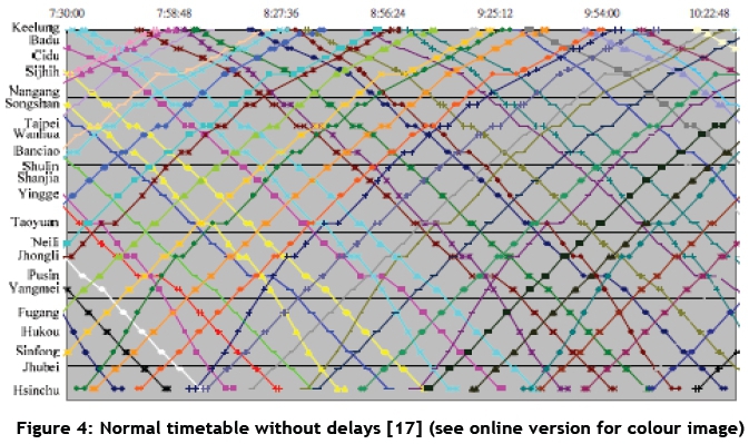
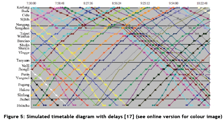
To validate their model, Hwang and Liu [17] used actual train operating data. The arrival-departure time data of a specific day was retrieved from the Centralised Train Control database of the Taiwan Railways Administration. Later, actual delay data was also collected in order to compare it with the simulation output. A route conflict delay was chosen as the real event that serves as the primary delay. The model proved to be within 120 seconds of the actual delay time 77.5 per cent of the time, and 62.5 per cent of the time it was within 60 seconds. Figure 4 shows the Marvey diagram of the normal timetable without any delays, and Figure 5 shows the diagram for the simulated timetable. It is clear that a delay occurred between Shongshan and Taipei stations, and that the next seven trains were affected by it.

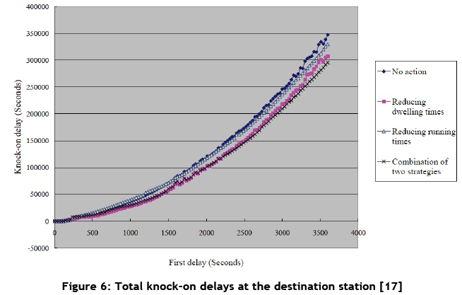
Hwang and Liu [17] went further and compared different delay reduction strategies and how they influence the total secondary delays; the effect of three strategies are shown in Figure 6. It is interesting to note the exponential relationship between primary (or first delay) and secondary delays (or knock on delays). This can be explained by the fact that the larger the primary delay is, the harder it is for a train to recover any of the lost time. A train is naturally limited by its ability to use these three strategies to recover the lost time created by the primary delay. A train has a minimum allowed dwell time at stations, and is also subject to speed limits on sections. These limitations thus translate into knock-on effects on later trains, which results in an exponential growth in the total delays.

Middelkoop and Bouwman [18] demonstrated the use of Simone simulation software to model the entire Dutch rail network. The software requires the following as inputs to the model:

• Infrastructure data.

• Timetable.

• Simulation-specific parameters.

• Network properties in relation to disruptions and disturbances.

• Operational rules.

• Statistical indicators for the simulation output.

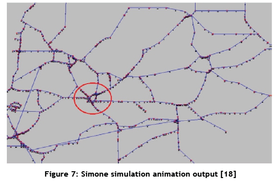
The software then produces the indicators pre-specified by the user and an animation of the network operation. Figure 7 shows an example of the animation output that Simone produces. The figure shows a part of the Dutch rail network and all the trains operating on it, with the red circle indicating a highly congested part of the network. Each type of train has a unique colour. Most parts of the model were constructed by the software's automatic model generator. The model included 600 stations, 1,100 track sections, and 350 trains, which is significantly large. The model was able to show, for example, the punctuality of trains in certain parts of the network and the relationship between initial delays and the sum of delays (as done by Hwang and Liu [17]).

 

 

Van Dijk [19] suggested that queuing theory and simulation can be combined. He argued that the advantages of queuing theory (e.g., generic components and few detailed data needed) reduce the disadvantages of simulation (i.e., high levels of complexity and the need for detailed data). In the same way, a simulation's advantages (i.e., real-life complexity and real-life uncertainties) reduce the queuing theory's disadvantages (i.e., over-simplification and unrealistic constraints).

Azadeh et al. [20] used a Visual SLAM coding language to develop a simulation model of a complex rail system consisting of 50 stations and both passenger and freight trains. An analytical hierarchy process (AHP) method was used to weight the qualitative and quantitative inputs and outputs, which were then converted to a data envelopment analysis (DEA). The objective of the model was to find ways to increase passenger train reliability and decrease the turn-around time of both passenger and freight trains.

Ho et al. [21] developed a general-purpose multi-train simulator that enables users to model without carrying out program code modifications. The simulator has been used in Hong Kong and China for studies of traffic control at conflict areas, scheduling optimisation, and the energy management of trains.

Train networks can be simulated in two ways. One is time-based modelling, where a time span is broken up into equal intervals and train movement is calculated at each interval. Although this is a very realistic representation of train movement, it requires a large amount of information with every update, which makes it computationally intensive. Time-based models are typically used in signalling layout design and energy consumption analysis [21].

The second way of simulating train movement is event-based. This method is similar to the queuing models discussed in Section 2.1. The train's movement is described in terms of a chain of events. For example, the train arrives at a station at a specified arrival rate and stays for a certain time period. The train then leaves and enters a track section, which marks the start of the next event. Each event's duration is characterised by a certain probability distribution. Although event-based models may reduce computational time significantly compared with time-based models, train movement updates are not synchronised between events [21].

 

4 CONCLUSION

This paper discussed the various ways to model and schedule train networks. First, purely analytical models were covered that showed that networks can be modelled accurately without advanced computational methods. They are, however, very limited in terms of scope and network complexity.

Second, heuristic methods were discussed. It can be concluded that these methods are very effective in optimising large complex networks. They allow the modeller to find global optima amid a solution plane consisting of many local optima. Optimising train schedules for dense rail networks seem to be possible with the right combination of these heuristic algorithms.

Last, the use of simulation was discussed. Simulation allows for very large scopes and even entire networks to be modelled [18]. It also has the ability to include important infrastructure detail and simulate reality fairly accurately. Moreover, it possesses the ability to animate the model, making the complex nature of a rail network visual and easier to understand.

The challenge is to combine these mathematical modelling techniques and simulation software to represent and predict real-life situations as accurately as possible. For future work, it is suggested that these techniques be applied to a case of the Passenger Rail Agency of South Africa (PRASA). In this case, PRASA has to introduce new and faster trains into a homogeneous rail system. The rail traffic will then become heterogeneous, implying that the network will have to be re-scheduled. The other issue is the following question: On which routes and in what quantity should the new trains be introduced so that service reliability will improve? The answers to this question can be estimated with the use of simulation modelling. Since most advanced simulation software available uses discrete events to model systems, and train operations can easily be described by discrete events, it is proposed to use discrete event simulation. Once a validated model is developed, heuristic methods can then be used to optimise the operation of trains in very specific scenarios. A very clear objective function and constraints are necessary, however, which could lead to a reduction of scope.

 

REFERENCES

[1] Kozan, E. and Higgens, A. 1998. Modeling train delays in urban networks. Transp. Sci., 32(4), pp. 346-357.         [ Links ]

[2] Gross, D., Shortle, J.F., Thompson, J.M. and Harris, C.M. 2008. Fundamentals of Queueing Theory. John Wiley & Sons        [ Links ]

[3] Huisman, T., Boucherie, R.J. and Van Dijk, N.M. 2002. A solvable queueing network model for railway networks and its validation and applications for the Netherlands. Eur. J. Oper. Res., 142(1), pp. 30-51.         [ Links ]

[4] Yuan, J. and Hansen, I.A. 2007. Optimizing capacity utilization of stations by estimating knock-on train delays. Transp. Res. Part B Methodol., 41(2), pp. 202-217.         [ Links ]

[5] Meester, L.E. and Muns, S. 2007. Stochastic delay propagation in railway networks and phase-type distributions. Transp. Res. Part B Methodol., 41(2), pp. 218-230.         [ Links ]

[6] De Kort, A., Heidergott, B., Van Egmand, R.J. and Hoogheimstra, G. 1999. Train movement analysis at railway stations: Procedures & evaluation of Wakob's Approach. 1st Edition, Delft: Delft University Press.         [ Links ]

[7] Burdett, R.L. and Kozan, E. 2010. A sequencing approach for creating new train timetables. OR spectrum, 32(1), pp.163-193.         [ Links ]

[8] D'Ariano, A., Pacciarelli, D. and Pranzo, M. 2007. A branch and bound algorithm for scheduling trains in a railway network. Eur. J. Oper. Res. , 183(2), pp. 643-657.         [ Links ]

[9] Burdett, R.L. and Kozan, E. 2009. Techniques for inserting additional trains into existing timetables. Transp. Res. Part B Methodol., 43(8-9), pp. 821-836.         [ Links ]

[10] Corman, F., D'Ariano, A., Pacciarelli, D. and Pranzo, M. 2010. A Tabu search algorithm for rerouting trains during rail operations. Transp. Res. Part B Methodol., 44(1), pp. 175-192.         [ Links ]

[11] D'Ariano, A., Corman, F., Pacciarelli, D. and Pranzo, M. 2008. Reordering and local rerouting strategies to manage train traffic in real time. Transp. Sci., 42(4), pp. 405-419.         [ Links ]

[12] Higgins, A., Kozan, E. and Ferreira, L. 1997. Heuristic techniques for single line train scheduling. J. Heuristics, 3(1), pp. 43-62.         [ Links ]

[13] Goldberg, D. and Holland, J. 1998. Genetic algorithms and machine learning, Mach. Learn., 3, pp. 95-99.         [ Links ]

[14] Chung, J.W., Oh, S.M. and Choi, I.C. 2009. A hybrid genetic algorithm for train sequencing in the Korean railway. Omega, 37(3), pp. 555-565.         [ Links ]

[15] Gorman, M.F. 1998. An application of genetic and tabu searches to the freight railroad operating plan problem. Ann. Oper. Res., 78, pp. 51-69.         [ Links ]

[16] Saayman, S. and Bekker, J. 1999. Drawing conclusions from deterministic logistic simulation models. Logist. Inf. Manag., 12(6), pp. 460-466.         [ Links ]

[17] Hwang, C.C. and Liu, J.-R. 2010. A simulation model for estimating knock-on delay of Taiwan regional railway. Journal of the Eastern Asia Society for Transportation Studies, 8, pp. 1110-1125.         [ Links ]

[18] Middelkoop, D. and Bouwman, M. 2001. Simone: Large scale train network simulations. 2001 Winter Simulation Conference, 2001(2), pp. 1605-1612.         [ Links ]

[19] Van Dijk, N.M. 2000. Hybrid combination of queueing and simulation. 2000 Winter Simulation Conference, 2000, pp. 147-150.         [ Links ]

[20] Azadeh, A., Ghaderi, S.F. and Izadbakhsh, H. 2008. Integration of DEA and AHP with computer simulation for railway system improvement and optimization. Appl. Math. Comput., 195(2), pp. 775-785.         [ Links ]

[21] Ho, T.K., Mao, B.H., Yuan, Z.Z., Liu, H.D. and Fung, Y.F. 2002. Computer simulation and modeling in railway applications. Comput. Phys. Commun., 143(1), pp. 1-10.         [ Links ]

 

 

Submitted by authors 16 Sep 2015
Accepted for publication 24 May 2016
Available online 12 Aug 2016

 

 

# Author was enrolled for an MEng (Industrial) degree in the Department of Industrial Engineering, Stellenbosch University, South Africa
* Corresponding author cjf@sun.ac.za