GENERAL ARTICLES

 

Estimating the continuous risk of accidents occurring in the mining industry in South Africa

 

 

A.F. van den Honert^I; P.J. Vlok^II

^IDepartment of Industrial Engineering University of Stellenbosch. andrew.vandenhonert@uniquegroup.com
^IIDepartment of Industrial Engineering University of Stellenbosch. pjvlok@sun.ac.za

 

 

---

ABSTRACT

This study contributes to the on-going efforts to improve occupational safety in the mining industry by creating a model capable of predicting the continuous risk of occupational accidents occurring. Contributing factors were identified and their sensitivity quantified. The approach included using an Artificial Neural Network (ANN) to identify patterns between the input attributes and to predict the continuous risk of accidents occurring. The predictive Artificial Neural Network (ANN) model used in this research was created, trained, and validated in the form of a case study with data from a platinum mine near Rustenburg in South Africa. This resulted in meaningful correlation between the predicted continuous risk and actual accidents.

---

OPSOMMING

Hierdie studie probeer 'n bydrae lewer om beroepsveiligheid in die mynbedryf te verbeter deur 'n model te skep wat in staat is daartoe om die voortdurende risiko's van moontlike werksongelukke te voorspel. Bydraende faktore is geidentifiseer en hulle sensitiwiteit is gekwantifiseer. Die benadering sluit in die gebruik van 'n Kunsmatige Neurale Netwerk (ANN) wat patrone identifiseer tussen die bydraende kenmerke en om die aanhoudende risiko van ongelukke te voorspel. Hierdie model was geskep, opgelei en gevalideer tydens 'n gevallestudie waar die data verkry is van 'n platinum-myn naby Rustenburg in Suid-Afrika. Die gevolgtrekking was dat 'n betekenisvolle korrelasie tussen die voorspelbare voortdurende risiko's en werklike ongelukke bestaan.

---

 

 

1 INTRODUCTION

In all forms of industry, employee safety is an essential aspect of the organisation's operations, regardless of the risks to which employees are exposed. The occurrence of an accident can be a violation of South African laws, can cost an organisation a lot in medical claims, and can result in a loss of productivity time and lowered employee efficiency [1]. There is a large knowledge gap in the field of predictive safety modelling, and this is the focus of this research.

The purpose of this research is to develop a model in the field of predictive modelling in a safety environment, dealing with the exposure of employees to known risks. Furthermore, this will add to the current lack in the body of knowledge about predictive safety modelling.

From the above discussion, the following null hypothesis, H₀, is derived:

H₀ A multivariate mathematical model cannot be used to link circumstantial variables to estimate the continuous risk of accidents occurring.

1.1 South African mine safety

Table 1 shows the statistics of accidents in the mining industry in South Africa in 2011 and 2012. A fatality rate and injury rate is included in the table, which indicates the rate of accidents per million worker-hours.

 

 

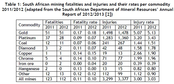
The South African Department of Mineral Resources [3] has established targets to reduce occupational fatalities and occupational injuries in the mining sector by 20 per cent per year over the period of 2013 to 2016. From Table 1, it can be easily seen that the gold and platinum mines are the largest contributors to mining fatalities and injuries in South Africa, with respect to the number of accidents occurring; these mines are also considered the most dangerous mining operations. Thus, in order to make the largest impact, the focus should be placed on reducing fatalities and injuries in the gold and platinum mines in South Africa. Furthermore, there are far more injuries than fatalities; thus the largest area for improvement would be in reducing the injuries within the gold and platinum mines in South Africa.

Clarke and Cooper [4] state that 60 to 80 per cent of all workplace accidents are due to work-place stress. Therefore, human behaviour is the biggest variable in industry and the source of the majority of risks. Organisations are continuously attempting to find ways to minimise the risks to which their employees are exposed. However, if these risks cannot be minimised, then exposure to the risks is minimised as identified by the HSE [5]. Although organisations do what they can to mitigate known risks by setting risk controls in place, such as elimination, substitution, engineering/design, administrative, and personal protective equipment (PPE), as well as regulations of how work is to be executed in the safest possible manner, it is impossible to eradicate them all. In light of this, an organisation is required to decide whether it is an acceptable risk, or whether different processes need to be put into place in order to bypass the risk. For example, automation in underground mines has been adopted to reduce the danger of 'fall of ground' (FOG) injuries.

For the purposes of this study, an accident refers to any undesired circumstances that give rise to ill-health or injury, whereas an incident refers to any near-misses and undesired circumstances that have the potential to cause harm.

There are five common injury classifications in the mining industry [12]:

1. Fatal injury (FI): an accident where an employee loses their life.

2. Serious injury (SI): an accident that causes a person to be admitted to a hospital for treatment for the injury.

3. Lost-time injury (LTI): an accident that occurs when an employee is injured and has to spend more than one complete day or shift away from work as a result of the accident.

4. Medical treatment case (MTC): any injury that is not an LTI, but does require treatment.

5. High potential incident (HPI): an event that has the potential to cause a significant adverse effect on the safety and health of a person; a near-miss is recorded as an HPI.

According to Bird [11], an accident triangle can be used to generalise the accident trends among themselves. For example, for every 600 incidents, there are 30 accidents, of which 10 are serious accidents and one is a fatal accident [11].

 

2 THE ARTIFICIAL NEURAL NETWORK PREDICTIVE MODEL

The model used in this research can be created in three separate parts: data manipulation for use in the network, training the model, and running the model to predict the continuous risk of an accident occurring in the future.

From research, multiple factors were found to influence the occurrence of an accident. However, since some of these factors are not measurable and some are measurable but not measured, the accuracy of the model is limited. Despite this limitation, the model has the ability to be extended easily to input additional influencing factors when they are measured. The influential factors that are measurable, and that were identified and measured in this study, are: location, occupation, noise level, time of day, time into shift, lighting, temperature, humidity, and production rate. This study did not include any HPIs in the predictive model because they are not actual accidents, and because there are many number of HPIs, and this would over-complicate the model. Thus, this model only included FIs, SIs, LTIs, and MTCs.

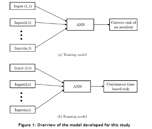
The first part of the model manipulates these values to prepare them as inputs for training the network. The next part takes these inputs and runs them through the Artificial Neural Network (ANN) model to calculate the current risk of accidents occurring. The third part of the model takes the ANN model with its associated parameters and uses the calculated current risk of accidents occurring. At this stage, the model also estimates future attribute values in order to predict the continuous risk of accidents occurring in the future, for the year with which the network was trained and for the subsequent year, in order to validate the network's accuracy within certain confidence intervals.

This model described above is presented schematically in Figure 1. Both the training and running models have 1-to-n inputs. However, the training model takes a vector of inputs at each accident, which results in a single risk value, whereas the running model takes a matrix of these inputs separated by a certain time interval, which results in a continuous time-based risk profile.

 

 

The model comprises an ANN model over multiple time steps, used together to predict future risk. The inputs to the model are the influential factors identified as causing accidents, which are normalised according to the distribution of accidents found.

2.1 Artificial Neural Networks (ANNs)

Russel and Norvig [6] state that ANNs have the aptitude to execute distributed computation, withstand noisy inputs, and learn. Even though Bayesian networks having the same properties, ANN persist as one of the most prevalent and effective forms of learning systems.

Larose [7] confirms that, with respect to noisy data, ANNs are robust because the network comprises multiple nodes, with every connection assigned different weights. Thus, an ANN can acquire the ability to function around uninformative examples in a dataset.

Nelles [8] and Page et al. [9] find that the most broadly-recognised and -used ANN architecture is the Multilayer Perceptron (MLP) network. This consists of one input layer, multiple hidden layers (usually one or two), and one output layer; this structure can be seen in Figure 2. Page et al. [9] add that the MLP network can accurately characterise any continuous non-linear function connecting inputs to outputs. Furthermore, Russel and Norvig [6] state that with one adequately-sized hidden layer, it is possible to represent any continuous function of the inputs with good accuracy; and with two hidden layers, even discontinuous functions can be represented. However, Russel and Norvig [6] find that very large networks generalise well if the weights are kept small, otherwise the large networks may memorise all the training examples and then not generalise well to new unseen inputs - a phenomenon known as 'over-fitting'.

 

 

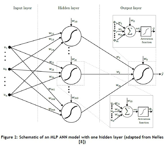
Page et al. [9] state that in an MLP network, the outputs of each node in a layer are linked to the inputs of all the nodes in the subsequent layer. For one hidden layer, as in Figure 2, the output neuron, ŷ, is a linear combination of the hidden layer neurons, ф¡, with an offset (or bias or threshold), w¡, which is expressed mathematically in Equation 1.

where:

m is the number of hidden neurons.

η is the number of inputs.

w¡ are the output layer weights.

w_ij- are the hidden layer weights.

U_jare the inputs.

Φ_j; is the output from the hidden layer neurons.

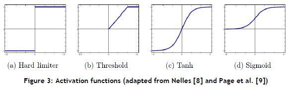
An activation function is a function that defines the output of a node. It scales the output value to a discrete value of '0' or '1' (hard limiter), or to a continuous value between '0' and '1' (sigmoid, threshold) or '-1' and '1' (tanh), depending on the function selected. These four activation functions, which are presented in Figure 3, are identified from the text. Of these activation functions, Russel and Norvig [6], Larose [7], Nelles [8], Page et al. [9], and Mitchell [10] all agree that the sigmoid (or logistic) function is the most common activation function used. Furthermore, Russel and Norvig [6] state that the sigmoid function is most popular because it is differentiable.

 

 

Page et al. [9] state that training the model using a set of input and output data determines the suitable values for the network weights (including the bias). Furthermore, Page et al. [9] state that training speed is influenced by the quantity of nodes in the network; therefore, the necessary quantity of nodes should be determined by the complexity of the relationships between the input and output data. They suggest using Principal Component Analysis (PCA) as a technique to measure the relative contribution of the inputs to output variations [9]. Additionally, they propose using the PCA values to initialise the weights for the model [9], although Mitchell [10] recommends initialising all the network weights with small random values between -0.5 and 0.5. This is in contrast to the numerous texts suggesting that the back-propagation algorithm is used for training the model, as it is the most popular technique. Mitchell [10] adds that multilayer networks trained with back-propagation are capable of expressing a large variety of non-linear decision surfaces. Mitchell [10] states further that the back-propagation algorithm for a multilayer network learns the weights using a gradient descent optimisation to try to minimise the squared error between the network output values and the target values for these outputs. Equation 2 presents the mathematical representation for the squared error between the network output values and the target values for these outputs.

where:

d is the training example.

D is the set of training examples.

k is the k^th output.

0 is the set of output units in the network.

t_kdis the target value of the k^th output and d^th training example.

o_kdis the output value of the k^th output and d^th training example.

Mitchell [10] adds that, in multilayer networks, multiple local minima can be found on the error surface, and the gradient descent search is only guaranteed to converge towards some local minima and not necessarily the global minimum error. Despite this, back-propagation still produces outstanding results. The back-propagation algorithm starts by creating a network with the preferred number of hidden and output nodes, and all weights are initialised. For each training example, it then applies the network to the example, computes the gradient with respect to the error on this example, and updates the weights in the network. This gradient descent step is then iterated until the network performs acceptably well.

 

3 SELECTION OF DATA ATTRIBUTES

The selection of data attributes required accident data. This was obtained from a platinum mine in South Africa, with the data spanning from 1st January 2009 to 31st December 2013. A detailed spreadsheet of the accident data, received from the mine for accidents over this period, contained the following attributes associated to each accident:

• Date.

• Time.

• Injury type.

• A description of the accident.

• Parent agency.

• Agency.

• Occupation.

• Task performed during accident.

• Body-part injured.

• Monthly production figures.

Furthermore, the South African Weather Service was approached for weather data for the area where the mines are located. The data received was for the same time period, and contained the following daily attributes:

• Daily maximum temperature.

• Daily minimum temperature.

• Daily humidity.

• Daily rainfall.

Since the received data covered numerous different occupations, it was not feasible to create separate models for each occupation. The data was therefore split into organisational groups, and a model was created for each grouping: underground, engineering, and other. This grouping was created on the basis of the data received: that the majority of accidents occurred in the underground section, whereas the engineering section had a significant number of accidents, and the rest of the organisational units appeared to have minimal accidents. Additionally, the 'task performed when the accident took place' and the 'body-part injured' attributes were not included in the model, as they would unnecessarily complicate it. Also, for the purposes of this model, any duplicate accidents were removed. Thus the remaining data attributes received were analysed, which included organisational units, parent agency, rainfall, humidity, time of day, temperatures, production rate, and seasonality.

 

4 DATA ATTRIBUTE NORMALISATION

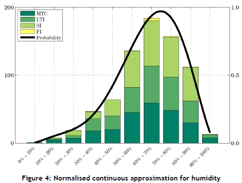
When comparing the effects that the various data attributes had on each organisational unit and the total dataset, it could be concluded that there was no significant difference between the total data distributions and the distributions of each of the three analysed organisational units (underground, engineering, and other) for each attribute analysed. As such, normalised continuous approximations were created for the input attributes, based on the total distributions. This was done in order to normalise the input data, as well as for ease of programming. Of the attributes analysed, the parent agency and seasonality were omitted, since no significant trends or deductions could be made from them. The rainfall attribute was also omitted because it would be programmed as a 'one' for rainfall and a 'zero' for no rainfall, and thus no normalisation was required for the rain. All of the normalised continuous approximations were plotted along with their associated distributions to see the correlation between the two.

Normalised continuous approximation plots were constructed for each attribute, where the left-hand y-axis represents the scale for the distribution of accidents, and the right-hand y-axis represents the scale for the normalised approximation. An example of this - that for humidity - can be seen in Figure 4. By visual inspection, the best fit curve to this distribution was found to be a 6^th order polynomial. Furthermore, the best fit curve for the time of day distribution was found to be a 10^th order polynomial. The best fit curve for the maximum temperature distribution was found to be a 5^th order polynomial, and the best fit curve for the minimum temperature distribution was found to be a 4^th order polynomial. Next, the best fit curve for the temperature difference distribution was found to be a 6^th order polynomial, and the best fit curve for the production rate distribution was found to be an exponential distribution.

 

 

 

5 DATA MANIPULATION

After the data had been split into three major sections - underground, engineering, and other - it was decided to train the model with 80 per cent of the data and validate it with the remaining 20 per cent. This corresponded to training with the first four years (20092012) and validating with the last year (2013). However, with the improvement of safety initiatives over the years, as well as organisational restructuring, this approach to the model did not yield adequate results. As a result of this, an alternative method was identified, which was to create a network for each year (in the range 2009-2012), and then validate each network with the subsequent year (in the range 2010-2013), thus creating four separate networks for each of the three sections. The various networks discussed above all refer to the same model discussed, but with different network weights associated to each model.

Next, 25 converse arguments were created to help train the model. These arguments were necessary due to the fact that if there were no examples in the data set for the network training that identify when no accident occurs, then the network would always generalise that for any inputs, the output would be an accident.

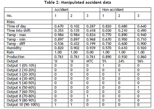
The model was used to identify patterns between the influencing factors for each accident (and converse arguments) and then to generalise the pattern that is used to identify the continuous risk. Due to this pattern recognition approach, the network makes use of a binary output classification system, is also known as a '1-of-n output structure'. The 1-of-n output structure for this model operates as follows: there are ten outputs that correspond to the output in units of 10 per cent (i.e., the first output refers to any output between 0 and 10 per cent, the second output refers to any output between 10 and 20 per cent, and so on). For example, if the first converse argument is 35 per cent risk, then for that training entry, all the cells are zero, except for the fourth cell, which is populated with a one. Thus the entire output matrix is populated with ones and zeros, and each example can only have a single 'one' in it. An example of this can be seen in Table 2, which is a sample of the training inputs and outputs to the network. With this system, the outputs for the converse arguments were ranged between the first seven columns, putting more emphasis on the lower risks because the accidents put the emphasis on the higher risks. The accidents were defined as follows: the output for an FI and an SI was assumed to be between 90 and 100 per cent; for an LTI, the output was assumed to be between 80 and 90 per cent; and for an MTC, the output was assumed to be between 70 and 80 per cent. This was done so that each category from 0 to 100 per cent had data points to train.

 

 

Next, all the data was manipulated according to the normalised continuous approximations discussed earlier, and the outputs were manipulated as mentioned above. Although no 'time into shift' data was received, it was assumed that there are two shifts, from 6h00 to 18h00 and from 18h00 to 6h00.

Continuous data for the five years (2009-2013) was similarly manipulated, but without any corresponding output values. The continuous data was broken down into two-hour segments for the entire five years; this was so that the 'time of day' and 'time into shift' had an influence on the network. For the temperature, humidity, and rainfall data, which was only recorded daily, the same values were used consecutively over the twelve two-hour entries, thus assuming that the entire day had the same conditions. However, this is not completely accurate, since the humidity would change throughout the day, or the rain might fall for only an hour or two of the entire day. However, this was the best generalisation that could be made with the available data. Furthermore, the production figures received were the monthly figures, not daily or hourly; thus every entry for the same month was assumed to be the same production value. Again, this is not completely accurate, but it was the best assumption that could be made with the available data.

 

6 TRAINING AND VALIDATION OF THE MODEL

Training and validation of the designed model is necessary to guarantee that the model functions as designed and to ensure the rigidity of the model. The training of the model was accomplished using Matlab's pattern recognition neural network tool. The processed data and the validation of the model took the form of a case study by observing and comparing the model risk outputs with the actual accidents.

A two-layer feed-forward neural network, with sigmoid hidden and output activation functions, was the network used in the model. This type of network can classify vectors well, given sufficient nodes in its hidden layer. For each network, the manipulated input values associated to the accidents and the converse arguments, as well as the target outputs, were loaded into the neural network pattern recognition tool in Matlab. On average, a data split of 70 per cent data for network training, 25 per cent data for network validation, and 5 per cent data for network testing was selected. These values were the best values found from trial and error.

Next step in the model setup was to set the number of hidden nodes. The number of hidden nodes was found, from trial and error, to be two-thirds of the sum of the quantity of input and output nodes, which yielded an adequate number of hidden nodes to use. This number corresponds to twelve hidden nodes, since there are eight inputs and ten outputs. Each network used started with twelve hidden nodes, but after many iterations, some models ended up requiring more hidden nodes.

Next, the network was trained numerous times and the best network was saved. It must be noted that training multiple times would generate different results due to different initial conditions and sampling. Furthermore, it must be noted that the lowest training error is not necessarily the best solution, as the network will not always generalise as well as a network with a slightly higher training error. A method could be to train with half the data and validate with the other half of the data until a suitable network approximates the entire data set, and this can be used for the model. When a suitable Mean Square Error (MSE) is reached, where lower values are better and zero implies no error, the re-training can stop. The total percentage error found in the confusion matrix indicates the fraction of samples misclassified; intuitively a value of zero implies no misclassification.

At this point, a confusion matrix can be plotted to check where the misclassifications occurred. This is done in order to identify whether any of the accidents are incorrectly classified, and whether the misclassification is minor (e.g., if an SI is classified as an LTI) or major (e.g., if an SI is misclassified as a 10 per cent risk). The confusion matrix has the network output on the y-axis and the target output on the x-axis. The main diagonal (from the top-left to the bottom-right) therefore indicates correct classification, and the rest of the blocks indicate misclassification. However, the blocks close to the main diagonal are minor misclassifications, and the further away from the diagonal, the greater the misclassification is. All misclassifications below the main diagonal are where the network predicts higher outputs than the targets. Above the main diagonal, the network predicts lower output values than the targets. An example of a confusion matrix can be seen in Figure 5 for the 2009 engineering network.

 

 

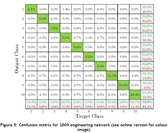
From this confusion matrix, it is seen that the majority of the data is correctly classified (along the main diagonal) and that the majority of the misclassifications are close to the main diagonal; this implies that they are close to their actual value. There are very few major misclassifications, and they mainly occurred through low target values being classified as a high output value. Since the majority of the misclassifications occur below the main diagonal, it is assumed the network will be biased more towards higher outputs. Of the classifications, 12.6 per cent occur below the main diagonal, and 8.4 per cent occur above the main diagonal; thus there is a bias of 4.2 per cent towards a higher output. This resulted in a classification accuracy of 78.9 per cent or a network training error of 21.1 per cent.

Once the errors have been found to be suitable, a model has been selected, and the confusion matrix is satisfactory, the network can be validated by running continuous data through it and comparing the output with the actual accidents.

The output of the model returns a vector of ten values for each step, which corresponds to the ten outputs. Every value in each vector relates to the correlation of each output; thus if there is a one in the tenth output, this implies that the model is certain that the output is an SI. However, if that value is 0.1, then the network is not certain that it is a SI. Thus, whichever output has the maximum correlation, it is assumed to be the output value. If the maximum value and second-highest value are close together, then no clear distinction can be made between the two categories. Thus for the purpose of this model, if the difference between the maximum value and second-highest value is more than or equal to 0.2, then the maximum value is used. On the other hand, if the difference between the maximum value and second-highest value is less than 0.2, then the average output between those two outputs is used. Next, the output is averaged to a daily risk value. Then the daily risk is plotted along with the actual accidents; this is performed for the current year of the model as well as the subsequent year. These continuous risk profiles can then be compared visually with the actual accidents in order to validate the model. Ideally, the risk should remain low and only peak when an accident occurs.

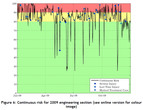
The continuous risk plots all have colour bands in the background to differentiate the various risk levels. These levels were set as 'high risk' for anything above 90 per cent (i.e., red), moderate risk for anything between 80 and 90 per cent (i.e., yellow), and acceptable risk for anything below 80 per cent (i.e., green). An example of a continuous risk plot can be seen in Figure 6 for the 2009 engineering section. From this plot, it can be seen that the continuous risk varies between 25 and 100 per cent, but that the majority if the risk lies above 80 per cent - as expected, given the number of accidents. The actual accidents that occurred in 2009 are plotted on the continuous risk line. This shows two major outliers that occur at 48 per cent risk. There are five accidents that occur just below the 80 per cent risk, but due to the random nature of accidents, it is assumed that there will be some outliers that cannot be predicted. Although there are sections where the risk is above 80 per cent and no accidents occurred, this does not imply an inaccurate model; the immeasurable component of human variability is also involved in the occurrence of accidents. Thus for exactly the same measured conditions, an accident could happen one day and not the next.

 

 

6.1 Sensitivity analysis

The sensitivity analysis was performed in three steps:

1. The mean values of each input attribute were calculated;

2. The network output for these mean inputs was computed; and

3. One input attribute at a time was varied to its maximum and minimum values, and the network output was computed for each scenario.

Figure 7 presents a box and whiskers plot of the outputs from the sensitivity analysis for each input variable. The solid black line is the average network output line. For each box, the whiskers represent the maximum and minimum outputs across all the networks. The top of the box represents the maximum average output per input attribute, while the bottom of the box represents the minimum average output per input attribute. Lastly, the mean value of each box is the mean value between the maximum and minimum average values per attribute.

 

 

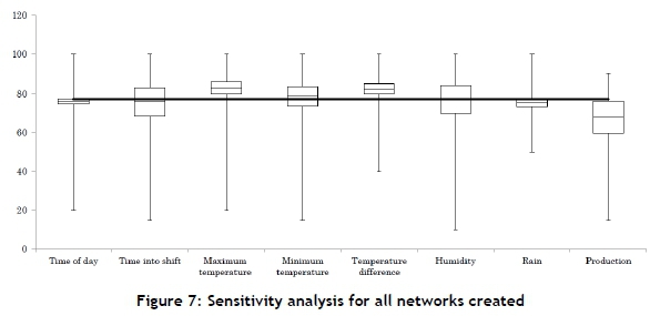
By ignoring the whiskers and looking only at the boxes in Figure 7, from the averages it appears that the production rate, humidity, and 'time into the shift' appear to have the largest influence on the network's output. Furthermore, it appears that the 'time of day' and rainfall have the smallest influence on the networks output.

6.2 Validation of network split

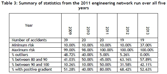
In order to identify why a network was created each year rather than creating one generic network, the 2011 network was used to predict the continuous risk profile for every year from 2009 to 2013 because it was the best engineering network. The number of accidents for each year was also overlaid on to these figures. It can be concluded that the networks are best-suited for the year for which they are trained and for the following year, but not for any other year. Table 3 shows that the 2011 trained engineering network is best suited for the actual data from 2011 and 2012, due to the lowest percentage of outliers and highest percentage of accidents actually occurring. The continuous risk profile is also a large positive value for 2011 and 2012 while the other years had much lower positive gradients. This confirms why a network is needed for each year that can be used to predict the following year, and not just one generic network that can be used indefinitely. Furthermore, it was identified from the results that it is not possible to draw any significant conclusions about the underground section of the mine because it is constantly at a high risk of having an accident.

 

 

 

7 USE OF THE MODEL

Now that the model has been trained and validated, the method for using the model can be discussed. First, future inputs will not be known, and so the entire year's continuous risk profile cannot be pre-determined because it was in the training and validation of the networks above. However, educated estimates of the next week's or month's temperatures, humidity, rainfall, and production rates can be identified and run through the model in order to output the next week's or month's risk profile.

The conditions are manipulated according to the normalised continuous approximations and then run through the underground, engineering, and other networks for the previous year. The networks can be updated continuously on a monthly basis, always using the previous twelve months of accident data for training. However, the further into the future that the inputs are estimated, the larger the chance of error.

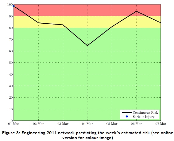
For the purpose of this example, the 2011 networks will be used. After the week's estimated data is normalised, it is run through the three networks; the output is plotted, and the actual accidents are included for reference. Figure 8 presents the week's continuous risk profile for the engineering section. From the plot, it can be seen that from the third to the sixth of March the risk is below 80 per cent, and is thus not an issue. Furthermore, from the sixth to the seventh of March, and from the first to the fourth of March, the continuous risk gradient is negative and so not as much of an issue. For the week predicted, the first of March is of concern (risk is 98%) and an accident did occur on the first of March. From the fifth to the sixth of March is also a concern, which is where the risk is above 80 per cent and the continuous risk profile has a positive gradient.

 

 

Grimaldi and Simonds [1] state that not all injuries can be prevented since they are unpredictable in nature, and that accidents do occur at times for reasons that are unpredictable. However, occupational injuries can be brought down to irreducible minimums.

This study has attempted to assist in highlighting high-risk time periods, where caution can be exercised in order to reduce the number of accidents occurring. The produced model worked well at estimating the continuous risk of accidents occurring across all sections of the mine. The results for the engineering section and other section were more useful, but the results from the underground section were not as useful because the risk was constantly above 80 per cent.

Despite the research objectives being met, there are still areas for improvement. Very few influential factors were used in the model due to the availability of data of many of the accidents. A recommendation is made to research more factors that influence accidents, and to identify and promote methods of measuring many of these factors on a continuous time basis. Such factors could include the number of hours slept the night before, lifestyle conditions (area of residence, number of people living together in residence, number of meals eaten per day, quality of life, etc.), experience at current job, and job satisfaction. Another recommendation is to determine a method that ensures that an optimal network is always selected when training the ANN, as settling on a suitable network is not always possible. Lastly, it is recommended that research is conducted into the probabilities linking the influencing factors to the inputs to the networks by making use of global statistics and using accident information from multiple industries; this could be more accurate than creating the probabilities from the histograms of the actual accidents.

It can be concluded that the null hypothesis can be rejected, and that this study was successful at creating a model that can be used to estimate the continuous risk of accidents occurring in the mining industry in South Africa. Additionally, due to the versatility of retraining the ANN, the model can easily be adapted and tested in different heavy industrial and labour-intensive industries.

 

REFERENCES

[1] Grimaldi, J.V. and Simonds, R.H. 1989. Safety management. 5^th edition, IRWAN.         [ Links ]

[2] South African Department of Mineral Resources. 2013. Annual report 2012/2013. Retrieved from: http://www.dmr.gov.za/publications/annual-report/summary/26-annual-reports/1020-annual-report-20122013.html        [ Links ]

[3] South African Department of Mineral Resources. 2013. Annual performance plan 2013/2014. Retrieved from: http://www.dmr.gov.za/publications/annual-report/viewcategory/26-annual-reports.html        [ Links ]

[4] Clarke, S.C. and Cooper, C.L. 2004. Managing the risk of workplace stress: Health and safety hazards. Routledge.         [ Links ]

[5] HSE. 1997. Successful health & safety management. Health & Safety Executive.         [ Links ]

[6] Russel, S. and Norvig, P. 2010. Artificial intelligence: A modern approach. Prentice Hall.         [ Links ]

[7] Larose, D.T. 2005. Discovering knowledge in data: An introduction to data mining. John Wiley & Sons.         [ Links ]

[8] Nelles, O. 2001. Nonlinear system identification - From classical approaches to neural network and fuzzy models. Springer.         [ Links ]

[9] Page, G., Gomm, J. and Williams, D. (eds) 1993. Application of neural networks to modelling and control. Chapman & Hall.         [ Links ]

[10] Mitchell, T.M. 1997. Machine learning. McGraw Hill.         [ Links ]

[11] Bird, F.E. and Germain, G.L. 1996. Practical loss control leadership, the conservation of people, property, process and profits. Det Norske Veritas.         [ Links ]

[12] Wannenburg, J. 2011. Predictive mine safety performance model based on statistical and behavioural science methods. MineSafe 2011. The Southern African Institute of Mining and Metallurgy.         [ Links ]

 

 

* Corresponding author
1 The author was enrolled for an a Master's degree in the Department of Industrial Engineering, University of Stellenbosch