GENERAL ARTICLES

 

Production uncertainties modelling by Bayesian inference using Gibbs sampling

 

 

A. Azizi^I; A.Y. bin Ali^II; L.W. Ping^III; M. Mohammadzadeh^IV

^IFaculty of Manufacturing Engineering University of Malaysia, Pahang, Malaysia Amirazizi'@ump.edu.my
^IIFaculty of Mechanical Engineering University of Science, Malaysia.meamir@usm.my,
^IIIFaculty of Mechanical Engineering University of Science, Malaysia.Meloh@usm.my
^IVDepartment of Statistics Tarbiat Modares University, Tehran, Iran mohsen_m@modares.ac.ir

 

 

---

ABSTRACT

Analysis by modelling production throughput is an efficient way to provide information for production decision-making. Observation and investigation based on a real-life tile production line revealed that the five main uncertain variables are demand rate, breakdown time, scrap rate, setup time, and lead time. The volatile nature of these random variables was observed over a specific period of 104 weeks. The processes were sequential and multi-stage. These five uncertain variables of production were modelled to reflect the performance of overall production by applying Bayesian inference using Gibbs sampling. The application of Bayesian inference for handling production uncertainties showed a robust model with 2.5 per cent mean absolute percentage error. It is recommended to consider the five main uncertain variables that are introduced in this study for production decision-making. The study proposes the use of Bayesian inference for superior accuracy in production decision-making.

---

OPSOMMING

Analise deur middel van die modellering van produksie deurset is 'n effektiewe manier om inligting vir produksiebesluitneming te verskaf. Die waarneem en ondersoek van 'n teélproduksielyn het getoon dat die vyf hoof onsekerheidsveranderlikes die vraagtempo, breektyd, skraptempo, opsteltyd en leityd is. Die vlugtige aard van hierdie toevalsveranderlikes is waargeneem oor 'n tydperk van 104 weke. Die prosesse was opeenvolgend en multi-stadium. Die vyf onsekerheidsveranderlikes van produksie is gemodelleer om die algehele vertoning van die produksie te weerspieél deur gebruik te maak van Bayesiese afleiding met Gibbs monsterneming. Die toepassing van Bayesiese afleiding vir die hanteer van produksie onsekerhede het 'n robuuste model, met 'n twee-en-'n-half persent gemiddelde absolute persentasie fout, tot gevolg gehad. Dit word aanbeveel dat die vyf belangrikste onsekerheidsveranderlikes, wat in hierdie studie bekendgestel is, oorweeg moet word vir produksiebesluitneming. Die studie stel die gebruik van die Bayesiese afleiding tegniek voor om sodoende beter akkuraatheid in produksiebesluitneming te verkry.

---

 

 

1 INTRODUCTION

Manufacturing industries should derive new approaches so that they can be agile and responsive in changing and uncertain manufacturing conditions, in order to survive the rapidly-changing and uncertain manufacturing environments of the 21st century [1]. The rapid rate of technology innovation and new customer expectations has caused production modelling to ignore many fluctuating variables, such as demand changes over time caused by product redesign and potential uncertainties due to rate variation, and the designs consisting of mixed variation [2, 3]. Machines and processes are subject to random failures, and time loss is incurred when a setup change is required for different product types. Machine failures, demand fluctuations, and setup changes are the major production uncertainties [4]. These uncertainties cause changes in pre-described breakdown time, setup time, scrap rate, and lead time, thus causing non-adherence to initial production planning. These uncertainties occur randomly, and their values are not easily predicted.

It is essential to evaluate and analyse the causes of disruption and the uncertain variables on the production line through better estimates using robust approaches. Production throughput is commonly considered in analysis and modelling to be an important measure of production line performance [5-7]. Production modelling in uncertain conditions becomes even more complex if the manufacturing environment includes multi-stage production on multi-products [8]. The challenge in multi-stage production is in the propagation and accumulation of production uncertainties, which affect the production throughput. Therefore, the insufficiency of models in analysing and tackling uncertainties in production is the main problem in trying to generate more accurate decisions on production throughput.

This paper emphasises the production uncertainties of modelling. The Markov Chain Monte Carlo (MCMC) algorithm for Bayesian modelling was used to produce an accurate model of production rate estimation, with scrap rate, setup time, breakdown time, demand, and manufacturing lead time as input variables.

 

2 LITERATURE REVIEW

Koh & Gunasekaran [9] stated that the significant uncertainty factors in manufacturing environments are demand changes, lead time variations, and breakdown of machines. Models for production planning that consider uncertainty make superior planning decisions compared with models that do not [10]. Deif & El Maraghy [11] showed through simulation that ignoring uncertainty sources leads to wrong decisions. Processing time and breakdown time affect the production throughput [7, 12]. Peidro et al. [13] described the process of uncertainty as a result of an unreliable production process due to machinery breakdown time. Researchers recently worked on different uncertainty factors in several different manufacturing industries using different approaches. For example, Stratton et al. [14] proposed the use of a buffer to manage uncertainty in production systems. Kouvelis & Li [15] worked on supply-demand mismatches, and believed that tardy delivery was caused by the uncertain lead time within a production system, which led to loss of sales. Their proposed methodology to manage lead time uncertainty assumed a constant rate of demand, and did not consider other production uncertainties. Deif & El Maraghy [11] examined the effects of three uncertainties: demand, manufacturing delay, and capacity scalability delay, where the manufacturing delay had the highest effect.

A linear regression model was applied to formulate the strategy, environmental uncertainty, and performance measurement [16]. Associations of material shortage, labour shortage, machine shortage, and scrap towards product late delivery were shown through analysis of variance, correlation analysis, and cluster analysis [17]. Chen-Ritzo et al. [18] stochastically examined the order configuration uncertainty, where a stochastic model was applied to represent the problem of aligning demand to supply in configure-to-order systems; they demonstrated the relationship of order configuration to the value of accounting uncertainty, using the sample average approximation method. Al-Emran et al. [19] examined the effect of uncertainty in operational release planning on the total duration, using Monte Carlo (MC) simulation. They concluded that every uncertain factor individually increases makespan, where the effect of any combination of uncertainty factors was larger than the summation of their individual effects.

Baker & Powell [20] presented an analytical algorithm to analyse and predict production throughput at unbalanced workstations, where the operation times of stations were random. Simulation method and approximation algorithm were applied to analyse throughput under uncertainties such as unreliable machines and random processing times [21, 22]. Alden [12] provided an analytical equation in a general case where there were two workstations in a serial production line. The workstations had unequal processing time, downtime, and buffer size, whereas Blumenfeld & Li [5] considered a serial production line including two workstations with the same speed and buffer size. Wazed et al. [23] considered a production system under machine breakdown and quality variation. They examined the effect of common processes on throughput and lead time using the WITNESS software, and found that changes in the level of common process in the system significantly affected production throughput and lead time.

Probabilistic analyses require analysts to have information on the probability of all events. When this information is unavailable, the uniform distribution function is often used, which is justified by Laplace's principle of insufficient reason [24]. A measurement of probability is considered as an interval or a set whenever uncertainty is impossible to characterise using precise measurement methods. Probabilities that quantify uncertainties are based on the occurrence of events. Measurements of uncertainty have been almost exclusively investigated in terms of disjunctive variables. A disjunctive variable has a single value at any given time, but it is often tentative due to limited evidence.

Spiegelhalter et al. [25] developed Bayesian inference using the Gibbs sampling software version 0.5 to solve complex statistical problems. Spiegelhalter et al. [26] defined a Bayesian approach as "the explicit use of external evidence in the design, monitoring, analysis, interpretation, and reporting of scientific investigations". The most modern method of Bayesian inference is clearly Markov Chain Monte Carlo (MCMC) [27], a widely used simulation tool for Bayesian inference, which is introduced by Tanner [28]. The popular MCMC procedure is Gibbs sampling, which has also been widely used for sampling from the posterior distribution based on stochastic simulations for complex problems [29].

 

3 METHODOLOGY

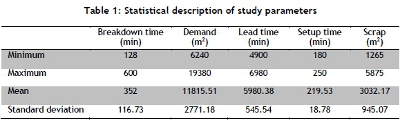
The case study data involving five uncertain variables - breakdown time, lead time of manufacturing, demand, setup time, and scrap - was collected through real-time observations and face-to-face interviews with the production line experts of a tile industry located in Qazvin, Iran. Altogether 104 weekly recorded data extracted from 20 highly requested types of tiles were used as the inputs for each uncertain variable to estimate the production throughput. These are statistically described in Table 1 and Figure 1.

 

 

 

 

For each uncertain variable, different continuous probability distributions were examined, such as uniform, exponential, and normal. Then from the prior probability distribution function, the posterior probability distribution function of the model parameters was computed. Different interpretations and justifications of non-informative (traditionally called 'uninformative') priors have been suggested over the years, including invariance - for example, [30, 31]. Nowadays, however, uninformative priors do not actually exist, because all priors are informative in some way[32]. Proper distributions with inverse gamma such as 0.001 for BUGS modelling were presented by [25, 26]. Weakly-informative prior (WIP) distributions are the most common priors in practice, and are favoured by subjective Bayesians because they use enough prior information for regularisation and stabilisation [33]. A highly popular WlP for a centred and scaled predictor is the normal distribution with a mean of 0 and a variance of 10000, which is equivalent to a standard deviation of 100, or precision of 1.0E-4 [25, 33, 34]. Statisticat [35] suggests a normal distribution with a mean of 0 and a variance of 1000 as a proper prior. The variance is dependent on the number of samples; if the sample is too large a variance of 10000 is a good choice. Hence, different variances for WIP were examined based on the experts' idea. Following Spiegelhalter et al. [25], the variances were fixed for the Bayesian model based on the smallest deviance information criterion (DIC) obtained. The DIC was introduced by Spiegelhalter [36] for model assessment as the most popular method of assessing model fit according to Statisticat [33]. DIC is the sum of the differences between the posterior mean of the model-level deviance and the complexity of model [36]. DIC measures the distance of the data to each of the approximate models, and is a better and simpler model [33]. Another non-informative prior distribution sometimes proposed in the Bayesian literature is uniform, which is not recommended by Gelman [34] because of its miscalibration. Thus, two different data sets of normal prior distribution are generated for each uncertain parameter of β, producing two chains to check for convergence.

The need to calculate high-dimensional integrals caused the Bayesian method for complex problems with several random parameters to become difficult. A sampling approach is proposed to overcome these difficulties. The popular procedure of MCMC, Gibbs sampling, was used to compute the Bayesian model. A generation of samples was examined to test the error of the model to reach the convergence by having five simulation runs: 1000, 5000, 8000, 10000, and 20000. For moderate-sized datasets involving standard statistical models, a few thousand iterations should be sufficient [37]. The model written was checked according to BUGS language. The checking showed that the model written was syntactically correct because the data was completely loaded, the model was correctly compiled, and the values were initially generated from distributions. Thus, the model was checked for completeness and consistency with the data.

In the Bayesian model (equation 1), all parameters are random, with normal distributions as priors while the variances are constant. The error term, denoted by e_t, has a zero mean and a constant variance that is statistically independent.

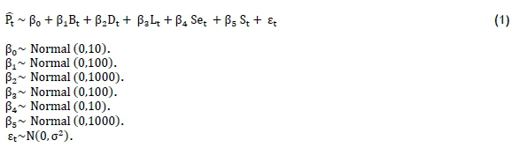
where

S_t= Scrap (1265 m²< S_t< 5875 m²)

B_t= Break time (128 min < B_t< 600 min )

D_t= Demand (6240 m²< D_t< 19,380 m²)

L_t= Lead time of manufacturing (4900 m²< L_t< 6980 m²)

P_t = Production throughput (5962 m² < Pt <19,000 m² ) β₀= Intercept

β₁..., β₄= Coefficient of variables (parameters of Bayesian model)

ε_t= Random error

The model generates valid results when the model presents convergence using a dynamic trace plot, autocorrelation function, and Brooks-Gelman-Rubin (BGR). The BGR diagnostic shows the convergence ratio[38]. The convergence showed graphically how quickly the distribution of uncertainty - for example β₁- approaches the conditional probability of p(β₁B_t). First checking was performed by visual inspection of trace/history plots. The model convergence was achieved when the two chains were overlapping. The convergence graphically shows how quickly the prior distributions of uncertainties approach the posterior distributions. Second checking was based on the autocorrelation test. The autocorrelation is defined between 0 and 1 or -1. A slow convergence of two chains graphically shows the high autocorrelation within chains. It implies that two chains are mixed slowly because true distributions are defined. Thus, the mixed or convergence chain contains most of the information to estimate an accurate posterior that indicates the validity of the model. The third check was done using the BGR diagnostic, which shows numerically the convergence ratio, which should be near to 1. The idea is to generate multiple chains starting at over-dispersed initial values, and assess convergence by comparing within and between chain variability over the second half of those chains. The model produces accurate estimations when it shows more efficiency based on lower MC error.

 

4 RESULTS

Table 2 presents the different variances of normal distributions and the calculated DIC respectively. Although set 1 resulted in lower DIC, as shown in Table 2, the other sets (different values given to the prior distributions) did not affect the DIC much. Thus, according to Bolstad [40], the prior is correct because it did not have a substantial effect.

 

 

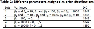
Figure 2 shows that the normal distribution is the best fit for the likelihood function of production throughput, with a 95 per cent confidence interval among the three other popular probability distributions - Weibull, logistic, and exponential.

 

 

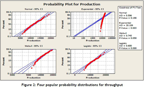
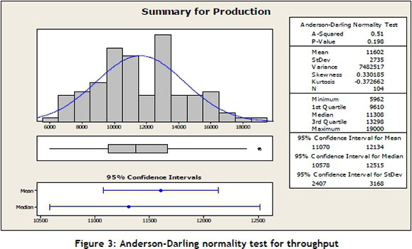
Figure 3 shows the descriptive statistics summary of a normal distribution function of production throughput with a mean value of 11602 and variance of 7482517. The Anderson-Darling normality test indicated the p-value of 0.198. This means that the data followed a normal distribution, because the p-value is greater than 0.05.

 

 

The regression model that was presented earlier in equation (1) is considered as the mean value of production throughput according to the Bayes theorem for the regression model [40], because the expectation vector is a linear function of a vector of the regression parameters (βί). Hence, the production throughput (output variable of the model) is distributed normally, according to the expectation vector and its scalar variance.

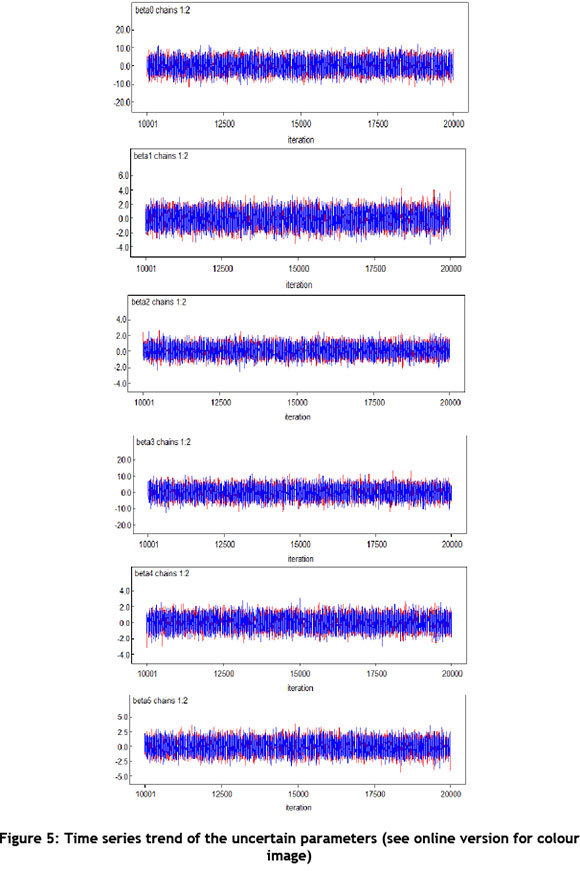
The Bayesian model was built after 20000 simulations for the situation under independent observation using BUGS software. The convergence diagnostics were checked through two obtained chains results. The chains show the generated samples in blue and red in Figure 4. Convergence was achieved because both chains overlapped each other[38]. The dynamic trace plots of the uncertain parameters are shown in Figure 4, with a 95 per cent credible interval.

 

 

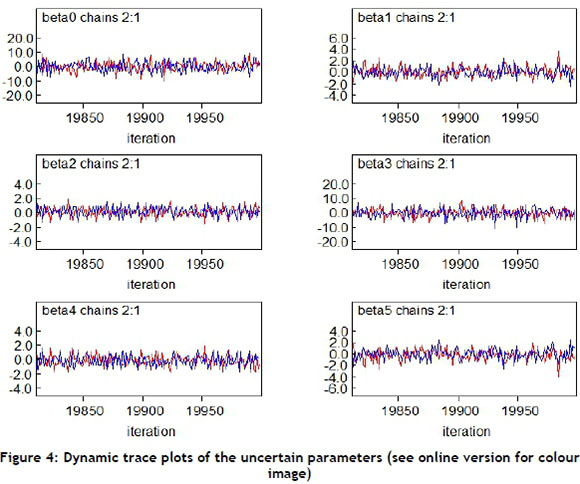
In Figure 5, there was no convergence problem because the chain looks like a fat hairy caterpillar[29, 41-43].

 

 

The autocorrelation functions for the chain of each parameter shown in Figure 6 indicated a gradual integrating of dimensions of the posterior distribution. Gradual integrating is often associated with high posterior correlations between parameters. The plots indicated that all parameters were integrated well, with autocorrelation vanishing before 20 lags for each case.

 

 

The BGR statistic was calculated for all five uncertain parameters using equation (2)[38]. The idea was to generate multiple chains, starting at over-dispersed initial values, and to assess convergence by comparing within and between chain variability over the second half of those chains.

where

W= width of the empirical credible interval of two chains based on all samples, andA= width average of the empirical credible intervals across the two chains.

The calculated value of BGR approached 1; thus the 20000 iterations were proven sufficient, and model convergence was achieved[41]. Figure 7 shows that the convergence of uncertain parameters approached 1 in all cases, especially after 12000 iterations. The BGR was depicted by the dotted line. W and A are properly overlapped to each other under the dotted line. It means that they are stabilised to tend to approximately constant value, which proves the model convergence[38]. This causes BGR (the dotted line) to come nearer to 1.

 

 

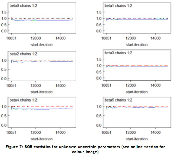
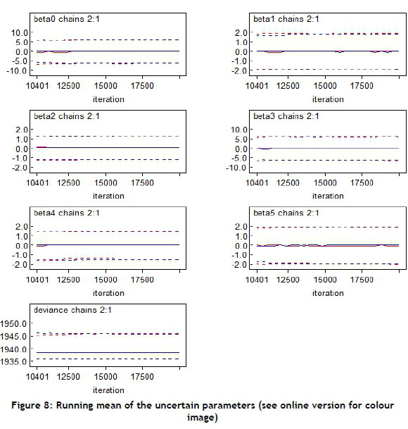
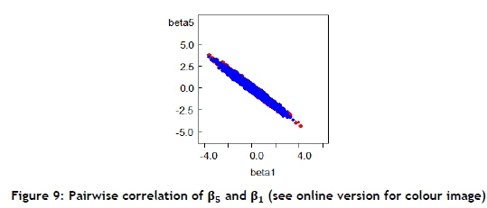
Figure 8 shows the running mean plots with 95 per cent confidence intervals after 1000 iterations. Bivariate posterior scatter plots present the correlation between two stochastic parameters. For example, Figure 9 shows the correlation between β₅and β₁

 

 

 

 

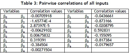
The values of the pairwise correlations between all parameters were calculated in Table 3. The highest value of correlations was between β₂and β₅, and the lowest value of correlations was between β₀ and β₃.

 

 

The estimated means of posterior distributions of the uncertain parameters (β_ί) were computed using Gibbs sampling and Bayesian rules with a 95 per cent posterior credible interval. The results are summarised in Table 4.

 

 

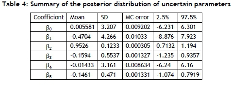
The lower value of MC error shows a more accurate model for Bayesian. The MC error for each unknown parameter is less than 5 per cent of the sample standard deviation. Finally, the Bayesian model is formulated in equation (3).

The outputs of the Bayesian model (equation (3)) were graphically compared with the actual throughput data to see any gap, as shown in Figure 10.

 

 

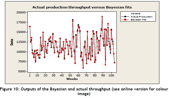
The Bayesian model shows a high level of efficiency for the estimated parameters of production uncertainties when the MC errors are less than 5 per cent of the standard deviation of coefficients, according to [39].

The value of the mean absolute percentage error (MAPE) of the Bayesian model was computed in equation (4) according to [44]. The value obtained was 2.5 per cent.

 

5 CONCLUSION AND RECOMMENDATION

Five significant uncertain variables in a dynamic manufacturing environment were modelled and analysed by applying Bayesian inference using Gibbs sampling. The Bayesian model results generated the posterior information on propagation of uncertainties and the relationship between them and the production throughput, with a 95 per cent credible interval under Bayes rules. The Bayesian model forecast production throughput under five production uncertainties with 2.5 per cent MAPE. The proposed Bayesian model provided a correct insight for the industrial planner and controller to decide how to match the production rate with production uncertainties when analytical solutions were unavailable. Therefore, researchers can concentrate on models of empirical relevance rather than models of convenient mathematical form.

 

ACKNOWLEDGEMENTS

This research is supported by the research university, Universiti Sains Malaysia under the Research University (RUI) Scheme (1001/ PMEKANIK/ 814188).

 

REFERENCES

[1] Gunasekaran, A. 1998. Agile manufacturing: Enablers and an implementation framework, International Journal of Production Research, 36, pp. 1223-1247.         [ Links ]

[2] Fisher, M.L. 2003. What is the right supply chain for your product?, Operations Management: Critical Perspectives on Business and Management, 4, p. 73.         [ Links ]

[3] Lee, H.L. 2002. Aligning supply chain strategies with product uncertainties, California Management Review, 44, pp. 105-119.         [ Links ]

[4] Fieldes, R. & Ingsman, B. 1997. Demand uncertainty and lot sizing in manufacturing systems: The value of forecasting: Working Paper MS 01, Lancaster University.         [ Links ]

[5] Blumenfeld, D.E. & Li, J. 2005. An analytical formula for throughput of a production line with identical stations and random failures, Mathematical Problems in Engineering, 3, pp. 293-308.         [ Links ]

[6] Li, J., Blumenfeld, D.E. & Alden, J.M. 2006. Comparisons of two-machine line models in throughput analysis, International Journal of Production Research, 44, pp. 1375-1398.         [ Links ]

[7] Li, J., Blumenfeld, D.E., Huang, N. & Alden, J.M. 2009. Throughput analysis of production systems: Recent advances and future topics, International Journal of Production Research, 47, pp. 3823-3851.         [ Links ]

[8] Du, X. & Chen, W. 2000. Methodology for managing the effect of uncertainty in simulation-based design, AIAA journal, 38, pp. 1471-1478.         [ Links ]

[9] Koh, S. & Gunasekaran, A. 2006. A knowledge management approach for managing uncertainty in manufacturing, Industrial Management & Data Systems, 106, pp. 439-459.         [ Links ]

[10] Mula, J., Poler, R., Garcia-Sabater, J. & Lario, F. 2006. Models for production planning under uncertainty: A review, International Journal of Production Economics, 103, pp. 271-285.         [ Links ]

[11] Deif, A.M. & El Maraghy, H.A. 2009. Modelling and analysis of dynamic capacity complexity in multi-stage production, Production Planning and Control, 20, pp. 737-749.         [ Links ]

[12] Alden, J. 2002. Estimating performance of two workstations in series with downtime and unequal speeds, General Motors Research & Development Center, Report R&D-9434, Warren, MI.         [ Links ]

[13] Peidro, D., Mula, J., Jiménez, M. & del Mar Botella, M. 2010. A fuzzy linear programming based approach for tactical supply chain planning in an uncertainty environment, European Journal of Operational Research, 205, pp. 65-80.         [ Links ]

[14] Stratton, R., Robey, D. & Allison, I. 2008. Utilising buffer management to manage uncertainty and focus improvement, Proceedings of the International Annual Conference of EurOMA, Gronegen, The Netherlands, pp. 1-10.         [ Links ]

[15] Kouvelis, P. & Li, J. 2008. Flexible backup supply and the management of lead time uncertainty, Production and Operations Management, 17, pp. 184-199.         [ Links ]

[16] Hoque, Z. 2004. A contingency model of the association between strategy, environmental uncertainty and performance measurement: Impact on organizational performance, International Business Review, 13, pp. 485-502.         [ Links ]

[17] Koh, S., Gunasekaran, A. & Saad, S. 2005. A business model for uncertainty management, Benchmarking: An International Journal, 12, pp. 383-400.         [ Links ]

[18] Chen-Ritzo, C.H., Ervolina, T., Harrison, T.P. & Gupta, B. 2010. Sales and operations planning in systems with order configuration uncertainty, European Journal of Operational Research, 205, pp. 604-614.         [ Links ]

[19] Al-Emran, A., Kapur, P., Pfahl, D. & Ruhe, G. 2010. Studying the impact of uncertainty in operational release planning: An integrated method and its initial evaluation, Information and Software Technology, 52, pp. 446-461.         [ Links ]

[20] Baker, K.R. & Powell, S.G. 1995. A predictive model for the throughput of simple assembly systems, European Journal of Operational Research, 81, pp. 336-345.         [ Links ]

[21] Han, M.S. & Park, D.J. 2002. Optimal buffer allocation of serial production lines with quality inspection machines, Computers & Industrial Engineering, 42, pp. 75-89.         [ Links ]

[22] Tempelmeier, H. 2003. Practical considerations in the optimization of flow production systems, International Journal of Production Research, 41, pp. 149-170.         [ Links ]

[23] Wazed, M.A., Ahmed, S. & Yusoff, N. 2010. Impacts of common processes in multistage production system under machine breakdown and quality uncertainties, African Journal of Business Management, 4, pp. 979-986.         [ Links ]

[24] Kass, R.E. & Wasserman, L. 1996. The selection of prior distributions by formal rules, Journal of the American Statistical Association, pp. 1343-1370.         [ Links ]

[25] Spiegelhalter, D., Thomas, A., Best, N. & Gilks, W. 1996. BUGS 0.5: Bayesian inference using Gibbs sampling manual (version ii), MRC Biostatistics Unit, Institute of Public Health, Cambridge, UK.         [ Links ]

[26] Spiegelhalter, D.J., Abrams, K.R. & Myles, J.P. 2004. Bayesian approaches to clinical trials and health-care evaluation, Vol. 13: Wiley, Chichester.         [ Links ]

[27] Koop, G., Steel, M.F.J. & Osiewalski, J. 1995. Posterior analysis of stochastic frontier models using Gibbs sampling, Computational Statistics, 10, pp. 353-373.         [ Links ]

[28] Tanner M.A. 1993. Tools for statistical inference, 2^nd edition. New York: Springer-Verlag.         [ Links ]

[29] Gilks, W.R., Richardson, S. & Spiegelhalter, D.J. 1996. Markov Chain Monte Carlo in practice. New York: Chapman and Hall/CRC.         [ Links ]

[30] Jeffreys, H. 1961. Theory of probability. Oxford University Press, UK.         [ Links ]

[31] Meng, X.L. & Zaslavsky, A.M. 2002. Single observation unbiased priors, Annals of Statistics, 30, pp. 1345-1375.         [ Links ]

[32] Irony, T. and Singpurwalla, N. 1997. Noninformative priors do not exist: A discussion with Jose M. Bernardo, Journal of Statistical Inference and Planning, 65, pp. 159-189.         [ Links ]

[33] Statisticat. 2012. LaplacesDemon: Complete Environment for Bayesian Inference, CRAN. R package version 12.         [ Links ]

[34] Gelman, A. 2006. Prior distributions for variance parameters in hierarchical models (comment on article by Browne and Draper), Bayesian Analysis, 1, pp. 515-534.         [ Links ]

[35] Statisticat. 2011. LaplacesDemon: An R Package for Bayesian Inference., R package version, 11.         [ Links ]

[36]Spiegelhalter, D.J., Best, N.G., Carlin, B.P. & van der Linde, A. 2002. Bayesian measures of model complexity and fit, Journal of the Royal Statistical Society: Series B (Statistical Methodology), 64, pp. 583-639.         [ Links ]

[37] Sheu, C. & O'Curry, S.L. 1998. Simulation-based Bayesian inference using BUGS, Behavior Research Methods, 30, pp. 232-237.         [ Links ]

[38] Brooks, S.P. & Gelman, A. 1998. Alternative methods for monitoring convergence of iterative simulations, Journal of Computational and Graphical Statistics, 7, pp. 434-455.         [ Links ]

[39] Roberts, G.O. 1996. Markov chain concepts related to sampling algorithms, Markov Chain Monte Carlo in practice, Chapman and Hall. London. UK.         [ Links ]

[40] Bolstad, W.M. 2004. Introduction to Bayesian statistics. Wiley-IEEE.         [ Links ]

[41] Gelman, A. 2004. Bayesian data analysis. CRC press.         [ Links ]

[42] Kruschke, J.K. 2010. Bayesian data analysis, Wiley Interdisciplinary Reviews: Cognitive Science, 1, pp. 658-676.         [ Links ]

[43] Goel, V. 2010. Application of an active comparator-based benefit-risk assessment in evaluating clinical trial design features of a new chemical entity using a Bayesian decision-theoretic framework. University of Minnesota Press. USA.         [ Links ]

[44] Chien, C.F., Hsu, C.Y. & Hsiao, C.W. 2011. Manufacturing intelligence to forecast and reduce semiconductor cycle time, Journal of Intelligent Manufacturing, pp. 1-14.         [ Links ]

 

 

* Corresponding author