GENERAL ARTICLES

 

Quantifying system reliability in rail transportation in an ageing fleet environment

 

 

P.D.F. Conradie^{I, *}; C.J. Fourie^II; P.J. Vlok^III; N.F. Treurnicht^IV

^IDepartment of Industrial Engineering Stellenbosch University, South Africa. pieterc@sun.ac.za
^IIDepartment of Industrial Engineering Stellenbosch University, South Africa. cjf@sun.ac.za
^IIIDepartment of Industrial Engineering Stellenbosch University, South Africa. pjvlok@sun.ac.za
^IVDepartment of Industrial Engineering Stellenbosch University, South Africa.nicotr@sun.ac.za

 

 

---

ABSTRACT

In recent years the management of physical assets has become increasingly important, especially in asset-intensive organisations. This article presents an approach to quantifying the reliability of rolling stock assets in the rail environment, making use of failure statistics. Failure distributions and the interdependency of different systems are used to determine the impact of component failures on overall system reliability, and to determine the reliability of individual train sets. Recommendations about the future planning of maintenance are included in the article.

---

OPSOMMING

Die bestuur van fisiese bates het in die afgelope tyd al meer belangrik geword, veral in bate intensiewe organisasies. Hierdie artikel stel 'n metode voor wat die betroubaarheid van rollende materiaal bates in die spoor bedryf kwantifiseer deur gebruik te maak van falingstatistiek. Falingverspreidings en interafhanklikheid van stelsels word gebruik om te bepaal wat die invloed is van komponent falings op die betroubaarheid van die totale stelsel. Hierdie benadering word dan gebruik om die betroubaarheid van individuele treinstelle te bepaal. Aanbevelings word ook gemaak hoe om betroubaarheid te gebruik om die beplanning van instandhouding te doen.

---

 

 

1 INTRODUCTION

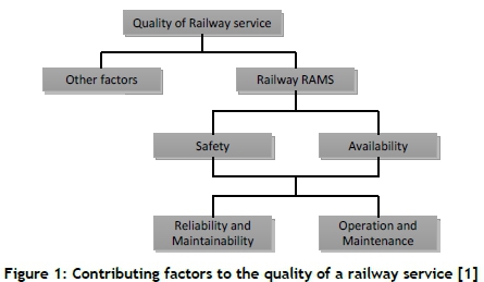
An effective rail system depends on the seamless integration of a number of complex systems. If one system fails, the whole service can be severely affected. Reliability, availability, maintainability, and safety (RAMS) are seen as major contributors to the quality of railway service (Figure 1), and are well covered in the European standard EN 50126 [1]. This standard recognises that railway safety and availability are interlinked and are regarded as the most important elements, and they can only be achieved if all the reliability and maintainability requirements are achieved. The quality of railway service is not only influenced by the four RAMS elements, but also by operations, maintenance, and other factors, as shown in Figure 1.

 

 

While all the elements of RAMS are important in the management of physical railway assets, in this article the focus will be on quantifying the reliability of railway rolling stock and the application of reliability techniques to define a forward-looking and leading reliability measure. As a case study, the method is applied using data from a South African rail operator that operates an ageing rolling stock fleet and predominantly makes use of time-based maintenance. Furthermore, the method for using the leading reliability measure in deciding on maintenance intervals will be discussed.

 

2 BACKGROUND

2.1 Concept of reliability

The word 'reliability' developed from the word 'rely', which is defined as a 'sense of dependence or trust and perhaps has a notion to fall back on' [2]. It was first used as early as 1816 by the poet Samuel T. Coleridge, who wrote about his friend who inspired everybody around him with "perfect consistency and absolute reliability" [3]. Since then the concept of reliability has become rather popular, and is used extensively by the general public as well by the technical community.

When used by the technical community, the context and interpretation of the word becomes rather specific, and can deviate substantially from the popular meaning. There are divergent definitions of 'reliability'; but one of the more appropriate and recently-used definitions in the context of asset reliability is "the probability that an item will perform its intended function for a specific interval under stated conditions" [1]. At first glance the definition seems to be self-explanatory, and misinterpretation appears improbable; but stakeholders need to ensure that the extent of intended function, the duration of the specific interval, and the scope of stated conditions are well understood.

Reliability analysis is a systematic approach to analysing the reliability of systems, identifying and accessing the frequency and causes of failures, and controlling the consequence of failures [4]. There are many reasons why reliability is important, such as reputation, customer satisfaction, operation and maintenance cost, repeat business, and competitive advantage [5]. But from a maintenance point of view, reliability will contribute to greater availability, which is particularly important in the context of RAMS.

2.2Reliability, availability, and the human factor

As part of RAMS, availability is seen as one of the most important reliability performance measures of maintained systems [6]. It is defined that the item must be "in a state to perform the required function under given conditions..." [1],[7]. The importance of reliability and availability in the rail industry is best described by Milutinovic [7], who quantifies the influence of reliability on availability. Reliability and availability are often misinterpreted, and in certain cases they are wrongly used as interchangeable terms.

Reliability can be grouped into the reliability of equipment and the reliability of people [8]. In EN 50l26 [1] the contribution of humans to railway RAMS is acknowledged, and more rigorous control of the human factors is called for. Studies have been done on human factors that include the influence of human reliability on systems. Karanikas [8] concluded that human errors contribute to more than three quarters of the failures during the life of an asset, and added that "expecting to achieve perfection from an imperfect human is unrealistic". Vanderhaegen [9] describes human behavioral degradation when performing tasks, and system degradation due to human actions. Without ignoring the importance of human reliability, in this article the focus will be primarily on the reliability of equipment, regardless of the cause of failure.

As stated, reliability is important, but it should not be pursued at any cost. Ultimately, the cost of reliability needs to be weighed against the total combined operation and downtime cost.

2.3Reliability and maintenance

Maintenance of industrial equipment is defined by Pintelon and Gelders [10] as "all activities necessary to restore equipment to, or keep it in a specified operating condition". The objective of maintenance is to maximise equipment availability by improving the reliability of the system [10] through scheduled preventative maintenance, replacements, and inspections (pMrI) [6]. Asset-intensive organisations should recognise the importance of an effective maintenance function. Sadly, however, in many organisations maintenance is seen as an expense account [11] and not as a value-adding process that is able to increase reliability.

Pham and Wang [12] realised that not all maintenance activities improve the condition of an item, and categorised maintenance according to the degree to which the operating conditions of an item is restored. They defined the following types of maintenance:

• perfect maintenance, which restores the operating condition of the system to as-good-as-new;
• minimal maintenance, which leaves the condition as-bad-as-old;
• imperfect maintenance, which leaves the system somewhere between the bad-as-old and good-as-new condition;
• worse maintenance, which causes a system failure rate or actual age increases without breakdown;
• worst maintenance, which unintentionally causes a failure or breakdown.

Possible causes identified by Pham and Wang [12] as 'imperfect', 'worse', or 'worst' maintenance include repairing the wrong part, partially repairing the fault, replacing with faulty parts, and human error.

It was believed by traditional maintenance practitioners that most failures of equipment were age-related, and a common mistake was to use a single maintenance strategy for all equipment. Failure models are often used to select the most appropriate maintenance strategies, and most of the six traditional failure curves for ageing equipment [13] can be managed by periodic time-based maintenance activities [14]. Some failures, however, cannot be prevented even by applying the best maintenance strategy, and these failures need to be predicted using statistical methods. This approach forms the focus of this article.

2.4 Reliability in the rail context

Many studies have been done on railway reliability and its effects, such as the relationship between reliability and productivity in railroad services [15], the importance of railway reliability to convince drivers of passenger vehicles to switch to public transport [16], the effect of unreliability on travel time [17], overcrowding because of delays and its effect on the productivity and efficiency of workers [18], and the effect of reliability on the availability of the service [7]. Railway reliability can be measured in different ways, such as the punctuality of the service [15], cancellations and delays [19], and the number of realised connections between trains [19].

From a passenger perspective, the punctuality of the service is often used as a reliability measure, defined as the probability that the train will arrive at the final destination within a certain margin of the scheduled arrival time. The average punctuality of some major European metro railroad operators is around 95 per cent [20], where trains arrive at the final destination within the international margin of five minutes, although some operators use a three-minute margin and still manage a punctuality of around 95per cent. In South Africa the punctuality of the Metrorail railway system was 84.5 per cent in 2011 [20] based on five minutes, which leaves room for improvement when compared with international benchmarks.

Studies clearly show that reliability is important to railroad companies, and the consequences of unreliability cannot be ignored. It is also clear that most reliability measures are based on the performance of the rail service, and that they are lagging indicators that cannot be related to the source of the unreliability. Lagging indicators show how well assets are managed, whereas leading indicators are forward-looking and help to manage the performance of an asset [8].

 

3 MODELLING RELIABILITY

3.1 Systems and theories

Calculating the reliability of a system requires a mathematical modelling of the system in terms of the underlying driving factors. When constant reliability values are used, a snapshot of system reliability is given at a specific time, and when time-dependent reliability expressions are used, the system reliability can be observed over a period of time [6].

Systems can be classified as non-repairable or repairable. A non-repairable system is discarded after its first failure [13],[21] and modelled using the renewal theory. With the renewal theory, the system is replaced after a failure and the condition is restored to the good-as-new condition, and failures are independent and identically distributed (i.i.d.). The renewal theory is not only limited to non-repairable systems, and even if a system can be physically repaired (defined as a repairable system) it can still produce failure data that is i.i.d., and can therefore be classified as non-repairable [22].

Normally a repairable system is not renewed to the good-as-new condition, but minimally repaired to the bad-as-old condition by the repair or replacement of the failed component(s) [13]. If the failure data has a trend, the condition of the system can deteriorate (or improve) over time, and must be modelled using regression techniques [13]. There is more about trend testing later.

The uncertainty associated with reliability can be classified as aleatory or epistemic uncertainty. Epistemic uncertainty represents failures caused by a lack of knowledge of the system, and it can be represented by mathematical structures such as interval analysis, possibility theory, evidence theory, and probability theory [23]. Epistemic uncertainty can be reduced by better understanding the system, such as by experimental results or physical models. Aleatory uncertainty is related to randomness, and is based on the mathematical structure of probability [23], which is the primary focus of this article.

3.2 Overview of system reliability and RBDs

For more comprehensive insight into the reliability of a system, it is important to be well-versed in the configuration of the system and the interaction between the system and its larger domain systems, as well as its peer systems, sub-systems, and components. Bourouni [4] describes a number of reliability assessment techniques, and compares the Reliability Block Diagram (RBD) to other reliability assessment techniques. He describes the RBD as the most logical and natural representation of a system, showing how units (components or subsystems) are logically linked in series, parallel, or combinations of units.

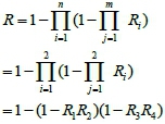
When units are linked in series, the failure of any unit results in system failure, and the reliability of a series system is the product of individual reliabilities, represented by

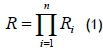where n is the total number of units in the system, R_i is the individual reliability values.

Units linked in parallel allow for redundancy, and the system remains operational even if only one unit is operational. The reliability of a pure parallel system can be calculated from individual unreliabilities, as shown below.

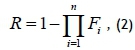where n is the total number of units in the system and F_i represents the individual unreliability of each unit defined as 1-R_j.

Unlike a pure series system, where the failure of a single unit results in system failure, or where a single unit needs to be operative in a parallel system, there are special variations where the system only operates when a certain number of units are operative in a certain sequence (k-out-of-n system) [5]. There are three variations of the k-out-of-n system, comprising the consecutive, balanced, and general k-out-of-n systems.

In the series configuration, the consecutive k-out-of-n system only fails if more than k consecutive units have failed [6]. In a balanced k-out-of-n system the failure of one unit can force the shutdown of another unit when in a particular arrangement [6]. In the general k-out-of-n system, redundancy can be built into parallel systems, where the system is operational when at least k units out of a total n units are operational, and the reliability of the system can be calculated as follows:

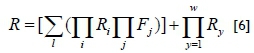
where l is the total number of possible combinations,

i : items required to survive

j : items allowed to fail

w : total number of units in the system

The general case of k-out-of-n systems is often adequate to model a system, and the pure series and parallel systems are special cases of the general case of k-out-of-n system. When the system is operational when only one unit is operational, it can be denoted as a general case of 1-out-of-n system, which in turn is a pure parallel system. When the system is only operational when all the units are operational, it is a general case of n-out-of-n systems simplified by a series system.

3.3 Reliability data and the selection of failure distributions

Reliability is regarded as the science of failures [4], and the purpose of the reliability engineer is to analyse trends in failure data and to determine the Rate of Occurrence Of Failures (ROCOF) as accurately as possible. The ROCOF represents the number of failures per unit time, and a common but erroneous approach of reliability engineers is to use only the mean time between failures (MTBF) in calculating the ROCOF, ignoring the chronological order of failure events. The result is that an assumption is indirectly made that failures occur randomly over the given period, and the opportunity to model failure trends is lost.

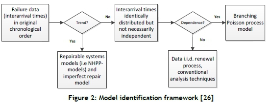
A practical model for the analysis of failure data, modified by Coetzee [24], is shown in Figure 2. It suggests that before a failure distribution can be fitted, failure data should first be tested for a trend; and if no trend is present, the dependency of failures should be determined. Vlok [25] comments that the test for dependence is most often omitted because a large number of failure observations are required to perform the test with reasonable confidence, and therefore independence is normally assumed.

 

 

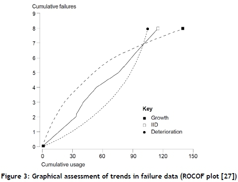
An informal graphical assessment of a trend in failure data is to plot the cumulative number of failures versus the cumulative system operating time. The graph is known as the ROCOF plot [27], and if the ROCOF is constant, the plotted points will be roughly aligned, and so the times between successive failures are identically distributed (marked ' I ID' in Figure 3). If the times between successive failures decrease, the curve presents a trend with larger increments in the number of failures per unit time, and the tail end of this curve indicates reliability deterioration (marked 'Deterioration' in Figure 3). Reliability growth is the opposite: it is when the times between successive failures increase, and the graph curves down with smaller increments in the number of failures per unit time (marked 'Growth' in Figure 3).

 

 

A simple trend validation can be performed by inspecting the data set using various techniques. The Laplace Trend Test (LTT) [13],[25] is the most extensively-used test for data sets, and was therefore chosen for this purpose. For failure data that ends in a failure, the trend parameter u can be calculated by:

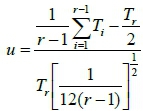where T₁,T₂,...,T_r = arrival times of failures, r = total number of observations [13],[25].

The null hypothesis (H₀) for the Laplace test is that the distribution of the arrival times corresponds to a Homogeneous Poisson Process (HPP) if the rejection criterion is met [28]. The rejection criterion is based on a standard normal distribution assumption, and it will reject H₀if u>z_a/2or u<-z_a/2[28]. Based on a typical 95 per cent confidence level (α=5%), H₀ will be rejected if u>1.96 or u<-1.96, and if u=0 it means that the trend is a horizontal line.

Coetzee [13] interprets the value of the Laplace value u in Table 1, and from the results the type of theory can be selected. Once either the renewable theory or the repairable system theory is selected, a family of distributions can be selected and the parameters determined by the most appropriate method.

 

 

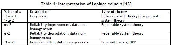
When the Laplace u value is within the grey area, further tests can be performed. Without discussing in detail the Lewis-Robinson test [28], Mann test [29], Weibull test or the Carroll-Hung method [30] can be used to determine whether the data has a trend.

As discussed earlier, systems can be classified into non-repairable and repairable systems. These will be discussed below.

3.3.1 Non-repairable systems

The failure data for a non-repairable system is i.i.d., based on the LTT test, and failures in the data set can be assumed to come from the same statistical distribution, independently of one another. The data is homogeneous, can be represented by various standard distributions, and the renewal theory applies.

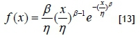
A variety of distributions can be used to model homogenous failure data. The Weibull distribution is one of the most commonly-used and flexible lifetime distributions [31], as shown below.

Substantial research has been done on more effective distributions, such as that by Unkle and Venkataraman [32], who found synergy between the Weibull and the Army Material Systems Analysis Activity (AMSAA) models. Xie and Lie [33] developed an additive Weibull distribution to represent the bathtub-shaped failure rate data with a single distribution that is related to the exponential and Weibull distributions. For the same purpose, Xie et al. [33] developed the new Weibull distribution, and when β<1, the lifetime data has a bathtub-shaped hazard rate function.

Similarly to the case of repairable systems, the reliability and related functions can be derived for the Weibull distribution. The exponential distribution, which assumes a constant failure rate, is a special case of the Weibull distribution with β=1 and λ=1 /η. It can be seen that the Weibull model is flexible and can be expanded or simplified. In the Weibull distribution, the β and η parameters can supply valuable information about the component in question.

The LTT has already confirmed that the life data is independent and identically-distributed, and the shape parameter (β) can indicate whether the hazard rate is increasing (β>1) or decreasing (β<1). The η is the characteristic life, which is an indication of the expected life and also an indication at what age 63.2 per cent of the components will fail [13].

3.3.2 Repairable systems

When a system is subjected to imperfect maintenance, it suffers from reliability degradation, with an increase in the ROCOF. These are repairable systems, represented by non-homogenous data, and can best be modelled by the non-homogeneous Poisson process (NHPP) [13],[24],[25]. The NHPP is generally suitable for the purpose of modelling data with a trend, relatively easy to use, and has been tested fairly well [24]. Two formats of the NHPP found in the literature are the log-linear NHPP, represented by

and the power law NHPP, represented by

The NHPP repairable systems are best modelled with α₁>0 (log-linear NHPP) and β>1 (power law NHPP), and a linearly increasing failure rate when β=2 (power law NHPP) [13]. System reliability, the expected number of failures, and MTBF can be calculated from the NHPP models, as shown in Table 2.

 

 

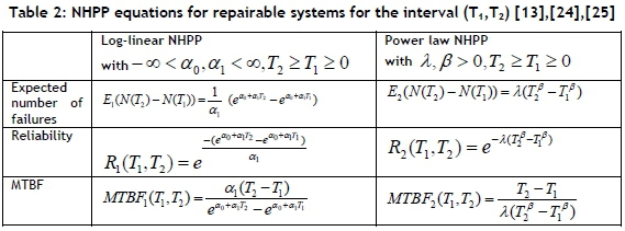
The estimation of the parameters from life data can be done using techniques such as the least-squares estimation (LSE) and the maximum likelihood estimation (MLE), and a test such as the Kolmogorov-Smirnov (KS) test can be used to determine the goodness of fit. However, this is not the primary purpose of this article, and it is not discussed further.

 

4 METHODOLOGY FOR MODELLING RELIABILITY

In the literature review, the importance of measuring and managing reliability is discussed, and different methods are discussed to calculate reliability. The methodology followed to calculate the reliability of a system is presented in this section, summarised in Figure 4.It consists of three steps, starting with the creation of the model, and ending with the interpretation of the results. Each step is discussed in more detail below, and is applied in the case study.

 

 

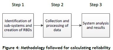
4.1 Step 1: Identification of systems and creating RBDs

The first step is to analyse the system, simplify the system, and identify the important subsystems. It is important that the contribution of sub-systems to reliability, their interaction with other sub-systems, and their redundancy be understood. The optimal assignment of components for every sub-system is also important, and the sub-systems must be balanced.

4.2 Step 2: Collecting and processing data

Once the sub-systems and components are identified, the best source of failure data must be identified, the data extracted, and analysis techniques used to determine relationships within the data sets (data mining). Techniques such as the Laplace trend test are used to search for trends in data sets, and failure distributions are then fitted to the data accordingly. Various software packages are available that can process data easily, but Microsoft® Excel was preferred for all the data processing.

4.3 Step 3: System analysis and results

Once the interactions of sub-systems are known, RBDs are created and failure distributions are determined for the components. The system can then be analysed. Again Microsoft® Excel was used to simulate the performance of the system over a period of time, and the contribution of components and sub-systems to system reliability could be identified.

 

5 CASE STUDY

The methodology is discussed in the previous section. It is now demonstrated by means of a case study, where the reliability of rolling stock at Metrorail (a subsidiary of the Passenger Rail Service of South Africa (pRaSA)) was modelled. Metrorail operates an ageing fleet of trains, some in operation since 1958, and they predominantly make use of cancellations and delays as reliability measures for their fleet [20].

5.1 Train set configuration

Metrorail defines a motor coach (MC) as a powered rail vehicle able to pull unpowered passenger trailers (PT) and also able to transport passengers. A typical Metrorail train set consists of nine PTs and three MCs, with an MC in the middle and at each end of the train set. The contribution of PTs towards the reliability of a train set is insignificant compared with the contribution of the MCs. Thus, for the purpose of this article, the train set is represented by three MCs only.

An MC consists of various sub-systems, configured in series and parallel. Although the subsystems have several components, a basic model was constructed demonstrating the interaction of four different sub-systems (refer to Table 3). Although a risk analysis, based on the impact and probability of occurrence, would have been more effective in identifying the components within each sub-system, the approach in this study is to construct a basic model where each sub-system is represented by a single component. The reasons for specifically selecting these components for the MC model are:

 

 

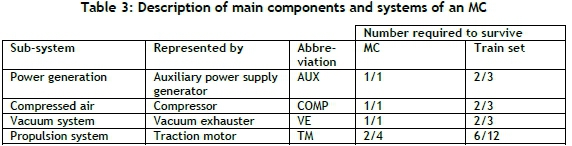
• each component is the main component in the respective sub-system;
• the components are either an electric motor or driven by an electric motor;
• these combined components contribute to more than 60 per cent of cancellations and delays of rolling stock at Metrorail [20];
• these components are serialised, repaired by Metrorail, and the failure data is available.

5.2 RBD models

Detail of the selected components is listed in Table 3, where the number of components required to survive in either an MC or a train set is indicated. The RBD of an MC is shown in Figure 5, which show the inter-relationship of the components and the redundancy.

 

 

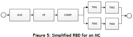
Most of the components are connected in series on an MC with redundancy only in the traction motors (TMs). The TMs are best described as a balanced k-out-of-n system represented by a series-parallel system, where each bogie on the MC is represented by two TMs in series. AN MC needs to have at least two TMs operating in series, which means that the failure of one TM will shut down the other TM on the same bogie.

By making use of equations (1), (2) and with individual reliabilities for each component, the reliability of the TM sub-system can be calculated as

where R=Reliability, R₁=Reliability of TM1, R₂ = Reliability of TM2, etc.

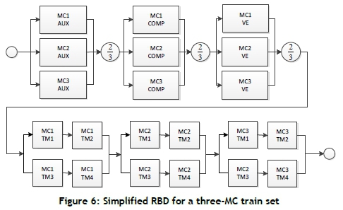
The RBD for a train set consisting of three MCs is shown in Figure 6. It can be seen that more redundancy is present in this configuration than in a single MC. The power generation, vacuum, and compressed air systems are best described as k-out-of-n systems, where two out of three sub-systems are required to be operational for the system to be functional.

 

 

5.3 Collecting and processing data

Once the logic of the sub-systems is understood and a RBD has been constructed, the failure characteristics of the different components can be calculated. Failure data from 2004 to 2013 was used from Metrorail's FMMS (Facility Maintenance Management System) to determine life distributions. The data represents nearly 200 MCs of the 5M-type train. It was reported by Metrorail that the data is incomplete, as the FMMS was not operating at times. Thus the assumption is made that the available data represents the real situation. For the purpose of this article, three MCs were selected with the worst failure data during the observation period.

For the sake of simplicity, failure data was limited to the replacement of components only -that is, perfect maintenance - ignoring any maintenance done in between the replacements. All components have one or more truncated failure observations (also called suspensions), where the last failure data points of the data set are not failures, but merely the end or beginning of the observation period.

The ROCOF graph for the exhauster of MC3 is shown in Figure 7. Three distinct periods are visible:

 

 

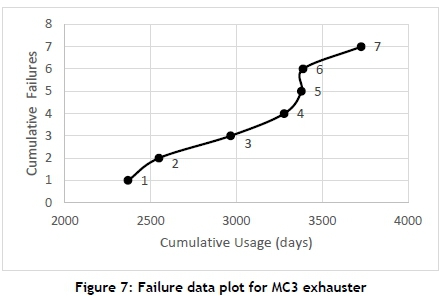
• Points 1 to 3, where reliability growth can be observed
• Points 3 to 5, deterioration period
• Points 5 to 7, reliability growth

The u factor for the LTT was calculated as 3.03, which indicates a strong overall reliability degradation trend over the observation period. So, although it seemed like the three periods were predominantly reliability growth periods, it is important to validate the data by performing trend tests.

The LTT is performed on the components of the three selected MCs, and where the LTT results were in the grey area, the Lewis Robinson and Mann tests were used. The same methodology is followed for all the MCs, but for the sake of simplicity only, the results for MC3 are reported in Table 4.

 

 

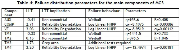
It can be seen that the compressor, vacuum exhauster, and traction motor 4 have reliability degradation trends. By using the LSE method, the data was fitted to either the power law NHPP or the log linear NHPP function. The LLT results were non-committal for the auxiliary equipment, traction motor 1, and traction motor 2. For these pieces of equipment the renewable theory HPP was followed, and the failure data fitted to the Weibull distribution using the linear regression method. The LTT results for traction motor 3 were in the grey area, and the Lewis Robinson test was not any more conclusive (U=1.55). Furthermore, with the Mann test, it was concluded that there was no trend (Mann Kendall Statistic=-7, Coefficient of Variation=1.12) and it was therefore concluded that the HPP with the Weibull distribution would be the best fit, and the Weibull parameters were calculated using the LSE (η=644.1, Β=0.764).

For each component, the KS test was used to determine the goodness of fit. The null hypothesis of the KS test states that the data follows the specified distribution, and it was rejected when the KS statistic (D_n) was greater than the critical value for the KS test (based on a confidence level of 90 per cent).

 

6 DISCUSSION OF RESULTS

An analysis was done of three individual MCs and a train set, made up of the three MCs. The results and a comparison of the reliabilities are reported in Figure 8. It becomes clear that the reliability of MC2 and MC3 follows a similar trend, with MC1 initially higher than MC2 and MC3, but then reducing to significantly less reliable than MC2 or MC3.

 

 

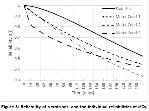
From the plot in Figure 8, the time period for a reliable life (also called warranty time) can be derived. Because of redundancy in the MCs, the reliability of the train set is higher than the reliability of any of the individual MCs. For example, the warranty time for the MCs over 14 days is 95.5 per cent for MC1, 94.8 per cent for MC2, and 83.0 per cent for MC3. The overall warranty time for the train set is 99.3 per cent over 14 days, which is higher than any of the individual reliabilities of the MCs. This shows, however, that this train set can only guarantee 99.3 per cent reliability over a 14-day period, which could have an impact on punctuality, cancellations, and delays.

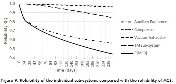
The reliability of MC3 shows an initial sharp decline. In Figure 9 the sub-systems of MC3 are shown, where it can be clearly seen that the auxiliary equipment has a significantly lower reliability than the other sub-systems. It follows a Weibull distribution with η=956.6 and □=0.408 and with such a low value, the steep reliability degradation can be expected.

 

 

At Metrorail the train sets are maintained every 14 days, and both the maintenance and operations departments expect a high level of reliability during the 14-day cycle. The train operations department, which operates the train sets, can quantify their expected reliability in terms of the percentage of successful missions completed, where a successful mission is defined as a train trip without failure.

This percentage of successful missions can be used by the maintenance department as a reliability target; and by using the reliability model described in this article, the reliability of the train sets could be quantified based on failure statistics, and compared with the reliability target.

 

7 CONCLUSION

Based on the results presented in this article, it can be concluded that system reliability for rolling stock in the rail environment can be successfully quantified. This reliability measure is a leading indicator, and the source of unreliability can be identified. Based on lifetime data and the interdependency of different systems, the overall reliability and the contribution of each component in the entire system can be calculated. It is also shown how time-dependent reliability expressions are used to study reliability over the life of the system.

Instead of using time-based maintenance, maintenance schedules can now be created based on the reliability of individual train sets. Train sets that meet the reliability target can be scheduled for maintenance less frequently than train sets that do not meet the target. Not only will the availability of train sets be higher, but the effort of the maintenance department will be focused on the less reliable train sets. This provides a different approach to maintenance management for ageing rolling stock fleets, and with the abundance of failure statistics, this method can contribute to RAMS in rolling stock.

 

FUNDING

This work was supported by Metrorail, a subsidiary of PRASA.

 

REFERENCES

[1] EN B. 50126. 1999. Railway Applications - The specification and demonstration of reliability, availability, maintainability, and safety (RAMS), British Standard.         [ Links ]

[2] Online Etymology Dictionary. 2014. Definition of 'rely', http://dictionary.reference.com/browse/rely. Accessed June 28, 2014.         [ Links ]

[3] Saleh, J.H. & Marais, K. 2001. Highlights from the early (and pre-) history of reliability engineering, Reliability Engineering and System Safety, 91(2), pp 249-256.         [ Links ]

[4] Bourouni, K. 2013. Availability assessment of a reverse osmosis plant: Comparison between reliability block diagram and fault tree analysis methods, Desalination, 313, pp 66-76.         [ Links ]

[5] Gulati, R. 2013. Maintenance and reliability best practices, New York, Industrial Press.         [ Links ]

[6] Elsayed, E.A. 2012. Reliability engineering. New Jersey, Wiley Publishing.         [ Links ]

[7] Milutinovic, D. & Lucanin, V. 2005. Relation between reliability and availability of railway vehicles, FME Transactions, 33(3), pp 135-139.         [ Links ]

[8] Karanikas, N. 2013. Using reliability indicators to explore human factors issues in maintenance databases, International Journal of Quality & Reliability Management, 30(2), pp 116-128.         [ Links ]

[9] Vanderhaegen, F. 2001. A non-probabilistic prospective and retrospective human reliability analysis method - application to railway system, Reliability Engineering and System Safety, 71(1), pp 1-13.         [ Links ]

[10] Pintelon, L.M. & Gelders, L. 1992. Maintenance management decision making, European Journal of Operational Research, 58(3), pp 301-317.         [ Links ]

[11] Tsang, A.H. 1998. A strategic approach to managing maintenance performance, Journal of Quality in Maintenance Engineering, 4(2), pp 87-94.         [ Links ]

[12] Pham, H. & Wang, H. 1996. Imperfect maintenance, European Journal of Operational Research, 94(3), pp 425-438.         [ Links ]

[13] Coetzee, J. 2004. Maintenance. Pretoria, Trafford Publishing.         [ Links ]

[14] Hashemian, H.M. & Bean, W.C. 2011. State-of-the-art predictive maintenance techniques. instrumentation and measurement, IEEE Transactions in 2011; 60(10):3480-3492.         [ Links ]

[15] Abate, M., Lijesen, M., Pels, E. & Roelevelt, A. 2013. The impact of reliability on the productivity of railroad companies, Transportation Research Part E: Logistics and Transportation Review, 51, pp 41-49.         [ Links ]

[16] Kingham, S., Dickinson, J. & Copsey, S. 2001. Travelling to work: Will people move out of their cars?, Transport Policy, 8(2), pp 151-160.         [ Links ]

[17] Rietveld, P., Bruinsma, F. & van Vuuren, D.J. 2001. Coping with unreliability in public transport chains: A case study for Netherlands, Transportation Research Part A: Policy and Practice, 35(6), pp 539-559.         [ Links ]

[18] Cox, T., Houdmont, J. & Griffiths, A. 2006. Rail passenger crowding, stress, health and safety in Britain, Transportation Research Part A: Policy and Practice, 40(3), pp 244-258.         [ Links ]

[19] Huisman, D., Kroon, L.G., Lentink, R.M. & Vromans, M.J. 2005. Operations research in passenger railway transportation, Statistica Neerlandica, 59(4), pp 467-497.         [ Links ]

[20] Conradie, P.D.F. & Treurnicht, N.F. 2012. Exploring critical failure modes in the rail environment and the consequential costs of unplanned maintenance, Computers and Industrial Engineering 42, pp. 76:1-76:13        [ Links ]

[21] O'Connor, P. & Kleyner, A. 2011. Practical reliability engineering. West Sussex, John Wiley & Sons.         [ Links ]

[22] Al Shaalane, A. 2012. Improving asset care plans in mining: Applying developments from aviation maintenance, Doctoral dissertation, Stellenbosch: Stellenbosch University.         [ Links ]

[23] Helton, J.C., Johnson, J.D., Oberkampf, W.L. & Sallaberry, C.J. 2010. Representation of analysis results involving aleatory and epistemic uncertainty, International Journal of General Systems, 39(6), pp 605-646.         [ Links ]

[24] Coetzee, J.L. 1997. The role of NHPP models in the practical analysis of maintenance failure data, Reliability Engineering and System Safety, 56(2), pp 161-168.         [ Links ]

[25] Vlok, P.J. 2011. Introduction to practical statistical analysis of failure time data: Long term cost optimisation and residual life estimation, Self-Published, Course notes.         [ Links ]

[26] Ascher, H. & Feingold, H. 1984. Repairable systems reliability: Modelling, inference, misconceptions and their causes, Lecture notes in Statistics. New York, Marcel Dekker.         [ Links ]

[27] Bohoris, G.A. 1996. Trend testing in reliability engineering, International Journal of Quality & Reliability Management, 13(2), pp 45-54.         [ Links ]

[28] Coit, D.W. 2005. Repairable systems reliability trend tests and evaluation. Proceedings of the Annual Reliability and Maintainability Symposium, pp. 416-421        [ Links ]

[29] Mann, H.B. 1945. Nonparametric tests against trend, Econometrica: Journal of the Econometric Society,Vol. 13, No. 3pp 245-259.         [ Links ]

[30] Leung, T., Carroll, T., Hung, M., Tsang, A. & Chung, W. 2007. The Carroll-Hung method for component reliability mapping in aircraft maintenance, Quality and Reliability Engineering International, 23(1), pp 137-154.         [ Links ]

[31] Xie, M., Tang, Y. & Goh, T.N. 2002. A modified Weibull extension with bathtub-shaped failure rate function, Reliability Engineering and System Safety, 76(3), pp 279-285.         [ Links ]

[32] Unkle, R. & Venkataraman, R. 2002. Relationship between Weibull and AMSAA models in reliability analysis: A case study, International Journal of Quality & Reliability Management, 19(8/9), pp 986-997.         [ Links ]

[33] Xie, M. & Lai, C.D. 1996. Reliability analysis using an additive Weibull model with bathtub-shaped failure rate function, Reliability Engineering and System Safety, 52(1), pp 87-93.         [ Links ]

 

 

* Corresponding author