CASE STUDIES

 

A stochastic analysis approach on the cost-time profile for selecting the best future state map

 

 

S.M. Seyedhosseini; A. Ebrahimi-Taleghani

Department of Industrial Engineering Iran University of Science and Technology, Iran. seyedhosseini@iust.ac.ir, aebrahimi@iust.ac.ir

 

 

---

ABSTRACT

In the literature on value stream mapping (VSM), the only basis for choosing the best future state map (FSM) among the proposed alternatives is the time factor. As a result, the FSM is selected as the best option because it has the least amount of total production lead time (TPLT). In this paper, the cost factor is considered in the FSM selection process, in addition to the time factor. Thus, for each of the proposed FSMs, the cost-time profile (CTP) is used. Two factors that are of particular importance for the customer and the manufacturer - the TPLT and the direct cost of the product - are reviewed and analysed by calculating the sub-area of the CTP curve, called the cost-time investment (CTI). In addition, variability in the generated data has been studied in each of the CTPs in order to choose the best FSM more precisely and accurately. Based on a proposed step-by-step stochastic analysis method, and also by using non-parametric Kernel estimation methods for estimating the probability density function of CTIs, the process of choosing the best FSM has been carried out, based not only on the minimum expected CTI, but also on the minimum expected variability amount in CTIs among proposed alternatives. By implementing this method during the process of choosing the best FSM, the manufacturing organisations will consider both the cost factor and the variability in the generated data, in addition to the time factor. Accordingly, the decision-making process proceeds more easily and logically than do traditional methods. Finally, to describe the effectiveness and applicability of the proposed method in this paper, it is applied to a case study on an industrial parts manufacturing company in Iran.

---

OPSOMMING

Volgens die literatuur oor waarde stroom kartering (VSM) is die tydfaktor die enigste rede vir die kies van die beste eienskap toestand kaart (FSM) bo die ander voorgestelde alternatiewe. FSM word gekies as die beste opsie omdat dit die kortste totale produksie lei tyd het. Hierdie artikel oorweeg die kostefaktor in die FSM seleksie proses saam met die tydfaktor. Dus, vir elkeen van die voorgestelde FSM kaarte word die koste-tyd profiel gebruik. Twee faktore wat van uiterste belang vir die kliënt en vervaardiger is, naamlik die totale produk lei tyd en die direkte koste van die produk, is hersien en analiseer deur die area onder die koste-tyd profiel kurwe te bereken. Hierdie area staan bekend as die koste-tyd belegging. Verder word veranderlikheid in die gegenereerde data bestudeer in elk van die koste-tyd profiele, sodat die beste FSM meer presies gekies kan word. Die beste FSM is bepaal deur 'n voorgestelde treë-vir-treë stogastiese analise metode en 'n nie-parametriese Kernel skatting van die waarskynlikheiddigtheidfunksie van die koste-tyd belegging. Die seleksie van die beste FSM is dus nie net op die minimum verwagte koste-tyd belegging gekies nie, maar ook op die minimum verwagte veranderlikheid van die koste-tyd belegging. Deur hierdie metode van FSM seleksie sal fabrikante beide die koste faktor en die veranderlikheid in die gegenereerde data, en die tyd faktor in ag neem. Dienooreenkomstig sal die besluitnemingsproses gladder en meer logies verloop as tradisionele metodes. Laastens, om die doeltreffendeheid en toepasbaarheid van dié voorgestelde metode te ondersoek, word dit toegepas op 'n gevallestudie van 'n industriële onderdele fabrikant in Iran.

---

 

 

1 INTRODUCTION

One of the production methods used by the most renowned companies in the world in recent decades is lean manufacturing. This concept was first introduced in the 1980s by a research group based at the Massachusetts Institute of Technology (MIT) who studied the Japanese way of production and the Toyota production system (TPS). As proposed by Womack and Jones [1], once a value is set for a specific product (the first principle of lean thinking), a value stream must be identified for that product (the second principle of lean thinking). Although identifying the total value stream for each product is a process that companies rarely attempt to conduct, it is usually through this phase that a surprisingly large amount of waste is revealed.

One of the most important and most applicable lean manufacturing techniques used to draw the value stream is value stream mapping (VSM). VSM is a graphical tool that uses a set of standard icons to map the processes in a production system. The technique was first developed by Rother and Shook [2] and was introduced in the book Learning to see. VSM, which is also called 'material and information flow mapping', demonstrates the sequence of material and information flow for the manufacturing processes, suppliers, and distribution of goods to the customers along the value stream. Thus VSM not only manages the manufacturing processes, but also optimises the whole system by creating a holistic view of it. While the main goal is to decrease the cycle time, the simultaneous illustration of materials and information flow helps the analyst in decision-making [3]. In the VSM, two types of mapping are used: current state mapping and future state mapping. A current state map (CSM) illustrates the current leanness level of the system, while a future state map (FSM) illustrates the future leanness level, which is what the system seeks. The time line drawn under the CSM and FSM shows the average time spent by an individual item in each phase of manufacturing processes.

In these processes, both value-added activities and non-value-added activities are included. The total achieved amount of time in each of the maps shows an estimation of total production lead time (TPLT) on each timeline. Both the TPLT and the ratio of total value-added time (TVAT) to TPLT IMAGEMAAQUI are two important parameters in lean manufacturing. Therefore, the identification of the time that it takes for an order to turn into a product and be delivered to the customer is vitally important for detecting and determining any waste in manufacturing processes. During the vSm, once the CSM and FSM are mapped and compared with each other, two main questions can be answered: (1) how lean is the current system? and (2) how lean can the system be in future? When these two questions are answered, improvements can be made to reduce waste in future processes. Maps are reviewed periodically, the improvement progress is tracked, and then the need for re-mapping is determined.

Since 2000, much research has been conducted on the application of VSM. For example, Dennis et al. [4] used simulation in conjunction with VSM to improve the performance of British Telecommunications PLC. Zahir et al. [5] stated that standard VSM has shortcomings in multi-product environments. To overcome this shortcoming, they developed value network mapping (VNM) for organisations with multiple products and value streams. VNM integrated some techniques such as production flow analysis, the simplification toolkit, and VSM. Duggan [6] introduced detailed procedures for using VSM in mixed model production systems. McDonald et al. [7] combined VSM with discrete-event simulation in order to determine the basic parameters of FSM and to evaluate the effects of these parameters on the performance of a production system. Pavnaskar et al. [8] determined the main differences and similarities of the engineering and manufacturing processes. The main goal of their research was to apply VSM in engineering processes. Braglia et al. [9] developed a new framework for using VSM in products with a temporised bill of material (TBOM).

Gurumurthy and Kodali [10] emphasised in their study that traditional VSM cannot be used for maintenance activities. Thus they developed a VSM specifically for maintenance in order to evaluate the non-value-adding (NVA) activities. These authors also provided recommendations to reduce the mean maintenance lead-time through simulation. Sobczyk and Koch [11] introduced the value stream cost map to measure the performance of value streams. Wu and Wee [12] applied VSM as a tool in the lean supply chain to analyse all the measurable indices that can be useful in cost reduction, quality increment, and lead time reduction through the Plan- Do- Check and Action PDCA improvement cycle. Lu et al. [13] identified uncertainty in customer demand as a noise factor using MCDM methods, hybrid Taguchi technique, and TOPSIS method, and then used VSM in order to visualise what conditions would pertain when improvements were applied.

Keil et al. [14] applied the value stream design technique to the semi-conductor industry, and considered flow necessities and variability management in all surrounding business processes. Jimenez et al. [15] applied the lean manufacturing principles to a winery, and showed that the VSM is one of the best tools for identifying possible improvements. Villarreal [16] adapted VSM to support efficiency improvement programmes in the transport operations environment. Rahani and Al-Ashraf [17] demonstrated the VSM techniques, and discussed the application of them to a case study on a product (Front disc, D45T).

John et al. [18] applied VSM in a machine manufacturing company. Their work included mathematical formulae that balance the work being performed to optimise the production resources necessary to achieve customer demand. Seyedhosseini et al. [19] proposed a method for identifying the critical value stream by using fuzzy set theory.

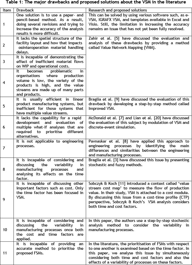
In our literature review of VSM, we found that, despite the many benefits of VSM, there are still problems and shortcomings. Some of these problems have been studied by researchers, while others are still being discussed. Table 1 indicates the major drawbacks and some of the research and solutions provided in this context. Some of the mentioned deficiencies are presented by Braglia et al. [3], while the rest are discussed by the authors of this paper.

One of the activities associated with VSM is to provide improvement methods from the proposed FSMs, followed by a CSM. After a review on the current situation, an organisation should propose various improvements once the shortcomings and weaknesses have been identified. However, it is important to note which of the FSMs is the most desirable, or on what basis the FSMs are being prioritised. Could FSM evaluations based only on time factors explain the real condition and uncertainties in production processes?

In this paper, we have investigated how the variability of processes affects the value stream when both time and cost factors are used simultaneously. After a stochastic analysis, the prioritisation of the recommended FSMs was analysed, based on a reduction in the expected variability found through the representation of an uncertain CTP.

Use of this method will cause the selection process of the most desirable FSM (compared with other proposed options) to be performed with greater accuracy and sensitivity. It is important to note that simultaneous evaluation of both time and cost factors in VSM in the form of CTP representation will help the organisation to meet the value defined by the customer. On this basis, both the production lead time and the direct cost of the product are consistently evaluated and analysed. This principle is of vital importance to both the customer and the organisation. Also, the selection of the most desirable FSM could prevent the high costs associated with implementation of the FSM, which might be the wrong choice and not be effective enough. It is important to mention that the selection of the most desirable FSM (compared with other proposed options) might not provide the same results if it is performed through the following two methods individually: time analysis and time-cost analysis.

On the other hand, with regard to variability in manufacturing systems, the complexity in evaluation and analysis processes might cause or increase the different results. However, it seems that once the cost factor and variability are considered, the accuracy in computations increases compared with conventional methods; on this basis, the decision-making process becomes easier and more logical.

Figure 1 illustrates the framework of this research. In order to explain the methodology used in this paper, the main concept of CTP is discussed briefly in Section 2.

 

2 THE CONCEPT OF THE COST-TIME PROFILE (CTP)

The basic concept of CTP was developed by the Westinghouse Corporation [21]. A CTP is a graph that shows the cumulative costs of a product spent per unit of time during each individual phase of its production. This graph shows the number of resources consumed from the beginning of manufacturing activities to the phase of invested resources recovery, when money is made by selling the product [22]. As mentioned by Rivera and Chen [22], a CTP graphs consist of several elements: activities, materials, wait, total cost, cost-time investment (CT), and direct cost. These elements are shown in the simple CTP graph in Figure 2, and are explained below.

 

 

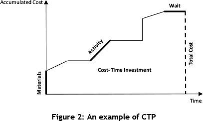
2.1 Activities

With regard to the activities in a CTP, two key assumptions should be considered. First, the related costs (excluding cost of material) are spent continuously and with a fixed rate during the ongoing activity. Second, the required materials for each activity should be prepared and made available before the activity begins. The activities in a CTP are represented as line segments with a positive slope. In fact, the activities in the CTP graph are shown based on the activity cost rate (ACR). ACR is the amount of money (in US$) spent for an activity during each unit of time. ACR is derived from the sum of the operator cost rate and the resource cost rate, which is composed of a depreciation charge and a maintenance charge [23].

2.2 Materials

In the CTP graph, materials are shown as vertical line segments because the materials are received instantaneously. When the materials are released for use in a process, their cost is added to the product cost, and is considered continuously as a part of the cumulative cost until the product is sold.

2.3 Wait

Sometimes no activities are performed in manufacturing processes; therefore the cumulative cost of the product will not increase at all. In the CTP graph, therefore. 'wait' is shown as horizontal lines. Although the 'wait' does not add any cost to the cumulative cost of the product, it is important because it increases the total time and causes delays in product sales. In other words, 'waiting' causes delays in the process of refunding the cost of resources spent in making the product.

2.4 Total cost

In the CTP, the total cost is represented by the height of the diagram once the production is complete and the product is sold to the customer. In fact, the total cost represents all the direct costs of the product that are incurred during the manufacturing process without yet considering the impact of the cost-time investment (CTI) and the time value of money [22].

2.5 Cost-time investment (CTI)

CTI, which is the area shown under the CTP, represents how much and how long the costs are accumulated during the manufacturing process. This area has implications for both time and cost factors. In fact, CTI refers to both the direct cost of the product and the budget of the company's working capital. It is also an indicator of the time value of money because it is, for example, better to spend US$20 and recover it in four days than to spend the same US$20 and recover one month later. CTI is the figure that will ultimately have an impact on the bottom line of the company and its financial management [23].

2.6 Direct cost

CTI is similar to any investment that an organisation can make and later demand for the investment return. Once the internal rate of return (IRR) associated with the carried investment (CTI) is applied, investment return can be evaluated. By taking the amount of investment made, considering IRR, and adding it to total cost, the direct cost can be calculated. However, the obtained direct cost represents the minimum amount a company should be able to recover after selling the product. On the one hand, the calculated amount of direct cost includes direct costs spent on the product, and on the other hand, it represents the time value of the spent costs over time [23]. Because the CTI is an actual investment, its cost can be calculated by multiplying it by the appropriate interest rate (IRR, cost of capital, cost of lost opportunities). The direct cost would then be the total cost plus the investment cost [22]. The following equation shows how the direct cost is calculated [22,23]:

In the next section we study variability and uncertainty in the CTP.

 

3 VARIABILITY IN THE CTP

To describe the variability in the CTP, it is best to discuss VSM first. VSM is a technique that was first used in the automotive industry, in an environment where the variety of products is limited. This technique operates more efficiently in an environment where the value streams are unidirectional and lack multiple production streams. Although one of the major and essential functions of VSM is collecting data, it has been observed that in most manufacturing systems, deterministic time data recorded on the timeline - whether during the process of identifying the current situation, or in the state of proposing the future situation - has always been problematic. To solve this issue in VSM and to determine time values with an uncertain nature, using conventional methods, we can consider the target values as the minimum and the maximum (with both optimistic and pessimistic attitude). Once the values are determined, based on the described method, the TPLT can be calculated. It is clear, however, that this approach cannot truly represent the amount of variability in manufacturing processes [3]. Thus variability, which is considered to be one of the main causes of disruption in planning the processes, should be carefully implemented and managed when the lean manufacturing principles are established [24].

It is worth noting that the variability that transfers from one process into another intensifies along the value stream and creates huge amounts of waste. So, with respect to high variability in processes, the possibility of having a levelled flow system would be minimised. The origin of the variability can come from all aspects of the value stream including, but not limited to, equipment, processes, work force, and product. Variability also affects the queue time and causes congestion and uncertainty in the input rates and the process [3]. In addition, variability is a significant noise factor for a pull system in processes, demands, random breakdowns, and random setup time [13].

Knowing that in VSM variability can only be examined in the time factor, if the cost factor is added a greater amount of variability can be observed. In fact, once the cost factor is entered in VSM, the simultaneous analysis of both time and cost will be presented in the CTP. This indicates that the variability in the CTP is much greater than in VSM. If it is well controlled and managed in the CTP, more precise results are achieved than if the variability is analysed only in the time factor. With respect to the above items and the importance of the variability, it seems that - before making any improvement in the system and moving forward to the proposed future state - it is necessary to analyse the variability in CTP.

In this paper, the variability in CTP will be analysed using stochastic analysis. Therefore the uncertainty in CTP, which is considered in association with the time factor, will be studied through the recommended stochastic analysis by considering the cost factor. In the next section, the intended stochastic analysis method is presented and discussed.

 

4 STOCHASTIC ANALYSIS ON CTP

Uncertainty analysis investigates the uncertainty of variables that are used in decision-making problems in which observations and models represent the knowledge base. In other words, uncertainty analysis aims to make a technical contribution to decision-making through the quantification of uncertainties in the relevant variables. One of the most common approaches to analysing that uncertainty is stochastic analysis. The main idea behind stochastic analysis is to describe values by probability density functions instead of by deterministic values. Hence, in VSM the time data with respect to an item spent at each stage of the value stream (process time, setup time, waiting time, transportation time, etc.) can be described with a probability distribution function. The stochastic analysis considered in this paper is used to compare the proposed FSMs. In other words, it is assumed that the organisation has mapped out CSM and, in order to improve the current state of affairs, plans to evaluate the proposed FSMs and choose the best option. The proposed approach in this paper can also be used for mapping out the CSM; but that issue has not been addressed here. Based on the proposed method presented by Braglia et al. [3], the literature review indicates that once the time factor in VSM is considered as value by probability density function and a comparison between the FSMs is performed, the FSM that has the lowest amount of variability among other proposed FSMs is recognised to be the best FSM.

According to central limit theorem, given x_x,x₂,x_nas independent random variables with the mean value of μ_i, the variance of σ_i² and Y = x₁ + x₂ +...+ x_n, then Y has a normal distribution with the mean value and the variance as in the following [25]:

It should be noted that this study was conducted based only on time as a factor. However, if the FSMs could be evaluated based on both time and cost factors simultaneously, the results would certainly be more useful for the organisation. In fact, use of CTP not only controls the factor of 'product delivery time to the customer', but also simultaneously controls and manages the factor of 'direct product cost' - a point of vital importance for both the customer and the manufacturer. In addition, using the central limit theorem in such a condition may be impossible or might present many challenges. Therefore other methods, such as non-parametric methods of estimating the density function, must be followed; these will be mentioned later in this paper. For a more detailed explanation of the stochastic analysis presented in this paper, the proposed approach is presented step-by-step, followed by a description of each section:

4.1.1 Step 1 - Applying the improved programme evaluation and review technique (PERT) for each interval

As already mentioned, we assume that, based on the CSM and weaknesses identified in the current state, several FSMs are suggested by production practitioners. As the first step, the density function of the different intervals on the timeline associated with each individual FSM should be estimated. Unfortunately, due to time and costs limitations, it is almost impossible to collect the required data, such as inventory levels and setup and cycle times, as random variables during VSM. Consequently, the identification of the probability function that best fits the experimental data is neither feasible nor convenient [3]. To do so, an improved programme evaluation and review technique (PERT) is used in this paper because it is both time- and cost-efficient.

PERT is a statistical tool used in project management, designed to analyse and represent the tasks involved in completing a given project. PERT is used commonly in conjunction with the critical path method. It enables us to incorporate uncertainty by making it possible to schedule a project while not knowing the precise details and durations of all the activities. Beta distribution can be used to model events, which are constrained to take place within an interval defined by a minimum and maximum value. So beta distribution with experimental mean and variance is used extensively in PERT. One reason to use beta distribution in PERT is that it enables us to handle skewness and easily apply it to the calculation of the activities' time mean value. The random variable of χ has beta distribution and is called a beta random variable if, and only if, its probability density would be as follows:

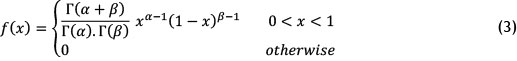
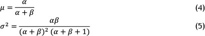
such that α,β > 0 and Γ(.) represents a Gamma function. Furthermore, the mean and the variance of beta distribution related to parameters (α,β) can be calculated using the following equations [26]:

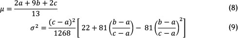
In PERT, however, shorthand computations are used widely to estimate the mean and standard deviation of the beta distribution:

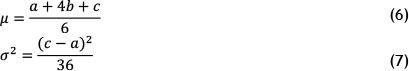
where is the minimum (optimistic estimate), is the maximum (pessimistic estimate), and is the most likely (realistic estimate) value. Using this set of approximations is known as a three-point estimation.

It should be noted that for each interval in an FSM, the parameters and should be sought and gathered from production practitioners. The above experimental mean and variance are not precise enough. A further improvement on the use of a beta distribution in PERT was done by Golenko-Ginzburg [27], who proposed a new experimental mean and variance with better and more precise estimations:

Therefore, in order to perform a more precise statistical analysis, we use Golenko-Ginzburg's [27] improved PERT for each interval. In association with each FSM, we are now in a stage where all the intervals ( ) are estimated as beta random variables with specific mean and variance, as follows:

4.1.2 Step 2 - Calculating the beta random variable parameters

Given the mean and the variance of intervals, beta distribution parameters ( , ) for each individual interval can be calculated based on the equations (4) and (5). The reason for doing this process is explained next.

4.1.3 Step 3 - Inserting the costly factors in FSMs and preparing a CTP for each proposed FSM

Up to this stage all the calculations and estimates have been done based on the time factor. In this stage, we now want to add the cost factor to the FSMs. Thus the associated CTP should be mapped for each FSM. So it is necessary to collect the related cost data, such as material cost and activity cost rate. It should be noted that, in order to avoid computational complexity, the cost values are assumed as certain values. However, according to the proposed method, considering both factors as uncertain values is also possible. As found in the literature, researchers usually use the time dimension alone in selecting the best FSM on the basis of the least amount of TPLT. In this paper, however, the simultaneous study of both time and cost factors will lead to more exact and more practical results. Thus, by mapping CTP for each individual proposed FSM, we can select the FSM that is in association with the least sub-area (CTI) compared with others. In fact, the FSM that creates the least amount of CTI represents the best condition, and is better than the other options.

4.1.4 Step 4 - Generating random beta numbers for each interval in each CTP

Another key objective of this paper is to estimate the probability density function of the sub-area (CTI) in order to enable us to evaluate the variability in different FSMs. To calculate CTI, it is necessary to perform algebraic operations such as addition, multiplication, and division on the time and cost data for each individual CTP. Figure 3 is an example of CTP, given here to show how the sub-area is calculated.

 

 

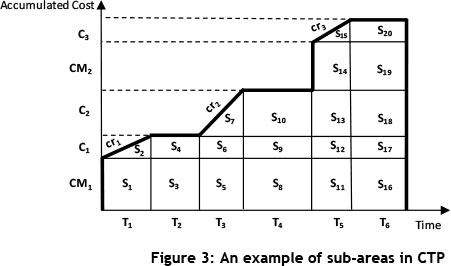
In this diagram, the following definitions have been used: 7_j , (j = 1,2 , ..., 6) shows the time interval.

CM_k ,(k = 1,2) shows the vertical line segment and indicates the cost of material.

cr_i;,(l = 1,2 ,3) shows the line segment with positive slope and indicates the activity cost rate.

C_m ,(m =1,2 ,3) shows the segment in the vertical axis (as a part of the accumulated cost), which is calculated from two elements: T_j and cr_l;.

As seen in Figure 3, CTI is obtained from the sum of all smaller areas, which are in the form of a triangle, rectangle, or trapezoid (S_t).

The way of calculating the CTI is vitally important due to the beta random variables, Assume that we want to calculate the two areas ₁and ₂. To calculate ₁, it is necessary to multiply the cost of material amount ₁by the time ₁. Accordingly, we have:

Thus the random variable ₁must be identified; this is obtained by multiplying a number by a beta random variable with specific mean and variance. This becomes possible once the random variable parameter ₁is identified through the required computations (which are not addressed in this paper).

Now, in order to calculate the area S₂, equation (14) must be followed:

Here one cannot easily determine what type of distribution S₂has. In fact, determining a variable distribution obtained from the multiplication of two dependent variables where both have beta distribution is not easily done. As can be observed, in order to determine other areas (S_t), we face similar challenges. For example, some of the areas are obtained by the multiplication of two independent random variables that each have a beta distribution. Thus it might no longer be possible to estimate CTI, which is obtained from the sum of all these areas, as a normal random variable with known parameters based on a central limit theorem.

However, due to the large number of required calculations, the high levels of computational complexity, and the uncertainty in determining the type of mentioned random variables (S_t) and relevant parameters, using this method seems to be very time-consuming. It can also be seen that, by considering the intervals as stochastic values and by assuming the cost values to be deterministic, the problem has faced such challenges. Obviously, once both the time and the cost factors are assumed to be uncertain, the problem will become more complex. Therefore, considering the above, and in order to compare the proposed FSMs in this paper, the above method has not been used. Instead, non-parametric methods are used to estimate the probability density function. Accordingly, in this stage for each interval in the mapped CTPs, an 'm' bits sample of random numbers is generated. Thus, we have:

4.1.5 Step 5 - Calculating the CTI in each CTP

Once 'm' variable numbers are generated for each interval in existing CTPs, the minor areas (S_i) and finally the corresponding CTI will be calculated. As a result, for each CTP 'm' number of CTI will be generated. Thus we have:

4.1.6 Step 6 - Estimating the probability density function of CTI

As explained in Step 4, the use of parametric methods to estimate the CTI probability density function causes problems and produces considerable computational complexities. In this paper, the kernel density estimate is used as a non-parametric method to estimate the CTI probability density function. Thus we have:

Next we explain briefly the methods (parametric and non-parametric) for estimating density functions, and in particular the method used in this paper. Thus we have divided this section into three parts. The first part explains briefly the concept of density estimation; the second part is related to the Kernel density estimator; and the third part explains some methods for proper bandwidth selection.

Estimation of probability density function

Many researchers during the past two decades have considered the subject of density estimation to be one of the most interesting topics. Density estimation has been used in various fields such as archaeology, banking, climatology, economics, genetics, and physiology [28].

Probability density function is the most fundamental concept in statistics, such that the random variable has a probability density function . When the function is specific, a natural description of distribution exists, which will allow the probability amount of to be calculated according to the following equation [29]:

Now imagine that we have a set of observed data points that are assumed to be a sample of an unknown probability density function. We therefore need to search for a method by which the probability density function can be estimated from the observed data. In this regard, two main approaches are discussed in the literature. In the first approach, which is called parametric density estimation, it is assumed that the data are selected from a known family of parametric probability distributions, such as the normal distribution with the mean (μ) and the variance (σ²). The density f underlying the data can then be estimated by finding estimates of ( ) and ( ²) from the data and substituting these estimates into the formula for the normal density [29].

The second approach is the nonparametric approach, which estimates the observed data distribution based on some assumptions. Although it will be assumed that the distribution has a probability density f, the data will be allowed to speak for themselves in determining the estimate of f more than would be the case if f were constrained to fall in a given parametric family [29].

As a nonparametric approach, we can consider methods such as histograms, Parzen windows, Kernel density estimation, and Naive Bayes classifier [28- 31].

Next, we briefly explain Kernel density estimation, which is the basis for density estimation in this paper.

A brief description for the Kernel density estimator

Assume x_l,x₂,...,x_nis 'n' bits sample of a random variable with density function ƒ. The kernel density estimate of f at the point x is given by

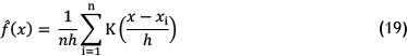
where K is a weighting function of a single variable called the kernel. The kernel K satisfies ƒ f(x)dx = 1, and the smoothing parameter h is known as the bandwidth. In general, any function having the following properties can be used as a kernel [28-31]:

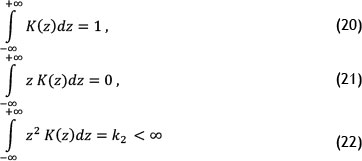
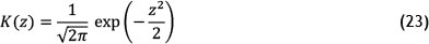
Different functions can be considered to be kernel functions. The most famous ones are Epanechnikov, Biweight, triangular, Gaussian, Silverman, and rectangular. Also, the most widely-used one is the Gaussian Kernel, which is defined as [28,30,32,33]:

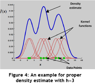
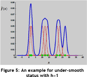
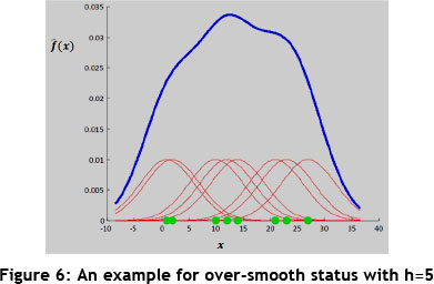
Kernel estimation of probability density functions is charactised by the kernel K, which determines the shape of the weighting function. The bandwidth h determines the 'width' of the weighting function and hence the amount of smoothing. The two components determine the properties of f(x) [29,30].

A large h will over-smooth the density estimation and mask the structure of the data, while a small h will yield a density estimation that is spiky and very hard to interpret. Figure 4 shows an example of how the Gaussian Kernel function is applied by selecting the proper h for a number of observed data point; it shows how the density function is estimated. Moreover, Figures 5 and 6 show the under-smooth and over-smooth states in density functions estimation based on considering small and large amounts for h respectively [29].

 

 

 

 

 

 

Proper bandwidth selection:

Various methods are found for bandwidth selection in the literature. Zucchini [30] proposed three main approaches to this topic that are briefly mentioned below:

1. Subjective selection

This method is based on testing and selection of different quantities for h and of the one that looks right in comparison with others.

2. Selection with reference to some given distribution

In this method, we must try to quantify the accuracy in density estimation. To do so, mean integration square error (MISE), which is considered to be a measure of the global accuracy of f(x), is used based on the following equations:

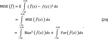
where the MSE measure is mean squared error.

Proceeding with the required calculations and using the Taylor series, the amounts of Bias (f(x)) and Var(f(x)), and as a result MISE(f), are identified as follows:

where j₂ = ƒ K(z)²dz and β (f) = ƒ f"(x) ²dx.

As observed in equation (27), for large values of h, the first term in (27) increases, and when h has small values, the second term in (27) increases. Thus, an optimal value of h makes the value of MISE(f) minimum.

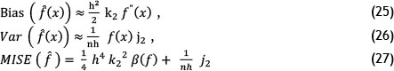
Now suppose we use the Gaussian Kernel to estimate density function. In this case:

where σ is the sample standard deviation and n is is the number of observed data points.

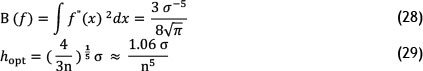
3. Cross-validation

In this method, the optimal bandwidth is determined as follows:

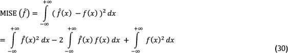
In equation (30), the third term has no dependency to the sample size and bandwidth. Accordingly, for the first and second term in (30), an approximately unbiased estimator is defined as follows:

such that f_-i(x_i) is the estimated density function of all of the data except x_i. When MCV(f) is calculated based on different values of h, the optimal value of bandwidth (h_opt) will be obtained from the value of h, which minimises the value of MCV(f).

In this paper, based on the method presented above, and by taking advantage of the Gaussian Kernel based on equation (29), the optimal bandwidth is determined using MATLAB software, and then the probability density function is estimated. The results are presented in the following sections.

4.1.7 Step 7 - Calculating the cumulative distribution function for CTI_h

Once the probability density function CTI has been estimated for each of the proposed FSMs based on the method presented in Step 6, we need to evaluate and prioritise the FSMs relative to each other. On this basis, by defining a critical area called 5*, the probability value Ρ (CTI < S*) for each of the FSMs will be identified. In other words, the cumulative distribution function will be estimated. In fact, P_h (CTI_h < S*) shows the probability that the CTI associated with the h^th FSM gets less than a specific area (S*). Hence, instead of choosing the FSM based on the minimum expected CTI, by calculating the value of Ρ we choose the FSM based on the largest value of probability, which indicates that the CTI would be less than a critical limit such as (S*). In other words, the obtained amount of probability enables the best FSM to be chosen based not only on the lowest expected CTI, but also on the lowest expected amount of variability in CTIs among the available options.

Thus the FSM that has the largest probability value will have the smaller CTI value, and will be in the first priority of selection. It can be said that the largest obtained probability value indicates that the associated FSM is better than the other FSMs in terms of product delivery time to the customer, and also in terms of the direct costs of the product. Accordingly, by obtaining the probability value in all FSMs, they can be prioritised relative to each other. In the next section, a relevant industrial case study is presented to assess the validity of the proposed approach.

 

5 MODEL IMPLEMENTATION IN AN INDUSTRIAL CASE STUDY

5.1 General information about the company

The research methodology was applied in a manufacturing company that produces the polymeric and metal parts for different industries, including automotive, transportation, and communication industries in Iran. This company was established in 1982 and is an ISO certified organisation that has received various quality awards.

The company has 150 employees, including workers, supervisors, engineers, and managers. Since the company's identity needs to be protected, we refer to it in this paper as the 'box manufacturer' (BM).

The company consists of four manufacturing shops:

Shop 1 : produces parts for the automotive industry;

Shop 2: produces parts for the transportation industry;

Shop 3: produces parts for the communications industry; and

Shop 4: works as a metal shop.

Shops 1, 2, and 3 are dedicated to manufacturing parts for the three industries mentioned above, while the last shop serves other shops with some required steel parts. The current research is focused only on Shops 3 and 4. In Shop 3, a wide range of communication products are manufactured. The shop is composed of two main sections:

1. The injection lines section composed of three separate production lines. Each line manufactures the required parts with respect to a pre-determined plan.

2. The main assembly line. The intended product family at the BM company is a postbox in the following two forms: 30-pairs and 50-pairs post-boxes. The product (the post-box) is made of polycarbonate, is resistant to ultraviolet, and is able to connect 30 or 50 participants (in 30-pairs or 50-pairs post-boxes respectively) simultaneously. The product's application is in cable telecommunication network projects. It should be noted that we have avoided proposing how CSM is achieved, or how the proposed FSMs are achieved, because the implementation of the method was presented in the previous sections of this paper. Below, the main processes in the production of post-boxes are specified:

(l₁)box holder injection line,

(l₂) box door injection line, and

(l₃) box frame injection line.

It should be noted that the streams I₁, I₂, and I₃ are located in the injection lines section of Shop 3.

(X) cutting, (Y) boring, and (Z) bending (stream XYZ) are located in Shop 4. Also, the main assembly stream consists of the following seven processes for assembling and completion of the product:

(A) box holder assembly;

(B) box frame assembly;

(C) stainless steel connecting holder assembly;

(D) assembling the box door into the frame;

(E) printing the product specification on the box door;

(F) final testing and quality control; and

(G) packaging.

5.2 CSM and the proposed FSMs

To map CSM, we need to gather some required data about information flow, machines, operators, and production flow, some of which are mentioned below:

The monthly order from customers for 30-pairs post-boxes and 50-pairs post-boxes is for 7,200 and 2,400 pieces respectively. There are 25 working days in each month, and each day includes two eight-hour shifts. Including two 24-minute breaks for each shift, the total available working time in each shift is equal to 25,920 seconds. The BM company asks its customers to place their orders 45 days before the expected delivery date of the order. Once an order is received, the relevant information is loaded into the material requirements planning (MRP) system, and the production planning manager plans for the production processes. In addition, daily production priorities are determined and announced by the production planning manager to the production supervisors. Based on these priorities, the supervisors determine the sequence of the production. Deviations in the customers' orders are also announced by the production planning manager via the MRP system to the production supervisors. (Customers usually finalise their orders one week before the delivery date.) Finally, the production planning manager announces the daily delivery programme to the delivery department. At the BM company, two main suppliers supply the required raw material: one supplies the required polycarbonate, and another supplies the stainless steel sheets that are required in the metal shop. The BM company's order quantity to the suppliers is determined by an economic order quantity (EOQ) model on a monthly basis. Each post-box product is packaged and put in a cardboard box after final testing and quality control. Every 12 boxes are then put on a big pallet. Every day 384 post-boxes (including 288 30-pairs post-boxes and 96 50-pairs post-boxes) must be produced and delivered to customers, based on their demands.

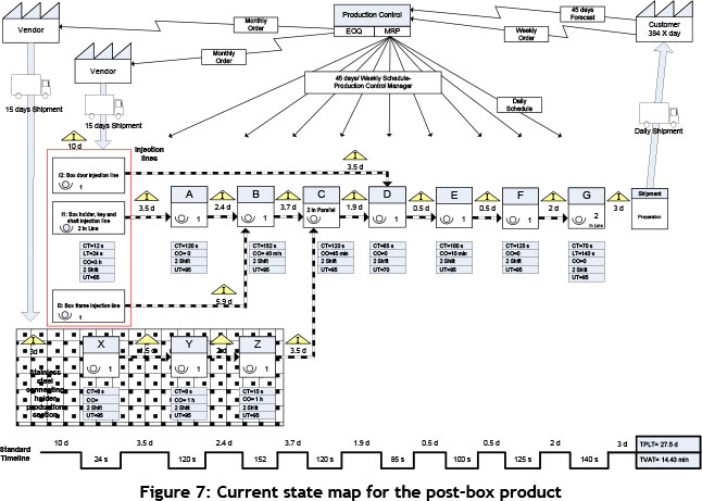
Considering that in post-box production multi-production value streams are observed, the critical value stream is focused on when mapping the current state. The modality of this selection is beyond the scope of this paper. Figure 7 shows the CSM for post-box production. Now, in order to improve the current state, the recommended improvements should be proposed by production practitioners and the VSM team in the form of FSMs once the weak points have been evaluated and identified. Therefore, before we select one of the FSMs and implement it using lean production techniques, it is necessary to choose the best FSM from the existing ones so that it results in the highest efficiency and the lowest cost in the production system. To produce a post-box based on CSM, the VSM team proposed FSMs after performing the necessary evaluations. It should be noted that the proposed suggestions are considered based on a takt time of 135 seconds and on operator-balance chart implementation and analysis.

For the sake of simplicity, we have proposed two FSMs. It is worth mentioning, however, that the method presented in this paper can be easily applied to more than two FSMs. Figures 8 and 9 show the recommended FSM1 and FSM2 respectively.

5.3 Application of the proposed approach in the BM company

At this stage, based on the steps explained in Section 4, we present the model and perform a stochastic analysis in association with FSM1 and FSM2. As can be seen in Figures 8 and 9, the TPLT for FSM1 and FSM2 in standard mode is equal to 6.5 and 6 days respectively.

At first it may seem that, because the TPLT is shorter in FSM2 than in FSM1, FSM2 should be selected as the better option, and all of the operational improvement activities should be performed on this basis in the production system. However, by applying the cost factor in VSM and evaluating the variability in corresponding CTPs, the useful results have been provided for decision-making. Thus we perform the proposed method based on the steps mentioned in Section 4, as follows:

5.3.1 Applying the first step

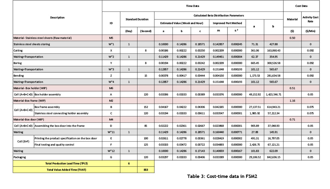
As mentioned in Section 4 (Step 1) the random variable X with beta distribution must have a value between 0 and 1. Accordingly, in order to identify parameters for each interval, the time values in days are converted into weeks, while the values in seconds are converted to hours, so that X can be estimated according to beta distribution based on the improved PERT. Once the optimistic, realistic, and pessimistic values for each interval are estimated, the mean and variance for each interval is calculated based on equations (8) and (9). The results can be seen in Tables 2 and 3.

5.3.2 Applying the second step

In this stage, based on equations (4) and (5), beta distribution parameters (α,β) are estimated for each interval of the FSMs. The obtained results can be seen in Tables 2 and 3.

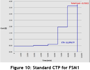
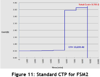
5.3.3 Applying the third step

So far, all calculations and estimations have been performed based on the time factor. At this stage, we want to map CTP for each FSM based on the cost factor. As seen in Tables 2 and 3, the required cost data, such as material cost and activity cost, are gathered and specified for each FSM. Once the necessary calculations are done, we map the CTPs related to each of the FSMs in the cases where the time and cost data are deterministic (standard CTP). Accordingly, the total cost values and sub-area (CTI) for each CTP are calculated. The obtained results can be seen in Figures 10 and 11. The results indicate that the total cost is equal for both CTPs. But the point is that the CTI related to FSM1 indicates less value than the CTI related to FSM2. However, if we compare the FSMs based only on the time factor, FSM2 represents better conditions than FSM1. Here, however, with the added consideration of the cost factor and the simultaneous evaluation of both time and cost factors in the FSMs, the circumstances were quite the opposite: FSM1 represents the more favourable conditions. As already mentioned, with the addition of the cost factor into the analysis, the level of computational accuracy becomes higher than in conventional methods, and the system situation is closer to reality. This result is obtained based on the CTP analysis in the cases where time and cost data were deterministic; if we analysed the variability in the data, the results might become different. This subject will be studied in the next sections.

 

 

 

 

5.3.4 Applying the fourth step

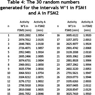
In order to increase accuracy and move toward the real conditions, the uncertainty in the data - in other words, the variability in the CTP - is studied. Thus, considering that in each of the CTPs each individual interval has a beta distribution with specified parameters, the random numbers are generated using Minitab 16 software. Accordingly, for each interval, a sample with the size of n = 30 random numbers is generated. This is done for each CTP individually. Table 4 shows the 30 random numbers generated for polycarbonate storing (W'1) activity in FSM1 with specific parameters (a = 198.07,β =481.07) and box holder assembly (A) activity in FSM2 with specific parameters (a = 49152.92,β = 1423546.71) as examples.

 

 

5.3.5 Applying the fifth step

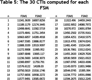
Once the 30 random numbers have been generated for each interval in each existing CTP, we calculate the minor areas (S_i) in them and then finally the related CTI. A sample of n = 30 random numbers is considered for each interval. Once the necessary calculations have been done, the number of 30 CTPs - in other words, the number of 30 CTIs - are generated for each of the FSMs, which are considered as data points. The computed CTI for each of the FSMs is shown in Table 5.

 

 

5.3.6 Applying the sixth step

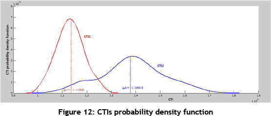
As some explanations of nonparametric methods of density function estimation have been proposed previously, this stage is based on kernel density estimation. By considering 30 generated CTI data points, CTI probability density function is estimated for each of the FSMs. Thus, using MATLAB software and by considering Gaussian kernel and calculating optimal bandwidth from equation (29), the probability density function is identified and mapped. It should be noted that the value of h for CTI₁(the CTI related to FSM1) and for CTl₂(the CTI related to FSM2) is obtained equal to 228.696 and 512.811 respectively. Figure 12 shows CTI probability density function for each of the FSMs.

 

 

5.3.7 Applying the seventh step

Once the CTI probability density function is estimated for each of the proposed FSMs in the previous stage, the CTI cumulative distribution function in association with each of FSMs is identified and mapped using MATLAB software. The corresponding results can be seen in Figure 13. Now we must evaluate and prioritise the FSMs relative to each other. On this basis, by defining a critical area called S*, the probability value Ρ (TCI < S*) for each of the FSMs will be identified; in other words, the cumulative distribution function will be estimated.

 

 

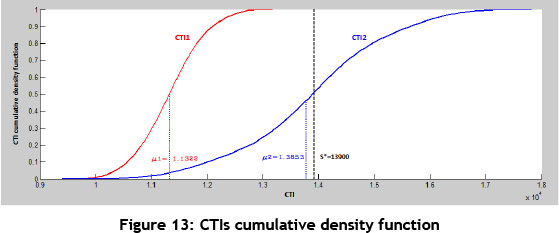
By defining S* = 13900, the targeted probability value in FSM1 and FSM2 is calculated as follows:

Ρ (CTI₁ < S*) = 1.000,

Ρ (CTI₂ < S*) = 0.5055

Considering that the obtained probability value in FSM1 is greater than that of FSM2, this means that the CTI (sub-area) related to FSM1 is smaller than that of FSM2, and is recognised therefore as the better option.

It should be noted that to select the best alternative for FSM1, we need to consider not only the expected reduction in CTI, but also the expected reduction in variability. Furthermore, the higher probability value in FSM1 suggests that this option, in terms of the simultaneous evaluation of the two factors of TPLT and direct cost of product, represents more favourable conditions than FSM2. Although the obtained results of selecting the best FSM are consistent with the results obtained from the standard CTP evaluation outlined in the previous sections, they could result in a different outcome.

 

6 CONCLUSION

By providing a step-by-step stochastic analysis, we have attempted to choose the best FSM from among proposed alternatives with more accuracy and sensitivity than by conventional methods. This paper has discussed the effects of variability in processes on the value stream, and how these effects can be analysed by simultaneously implementing both time and cost factors.

In this paper, the improved PERT has been used to estimate the probability density function of each interval in each of the FSMs. The cost factor in each FSM has then been entered through CTP mapping. Next, the probability density function of the CTP sub area, the CTI, has been estimated based on the non-parametric kernel estimation method. After this stage, the prioritisation of the proposed FSMs relative to each other has been evaluated by providing the uncertain CTP and calculation of distribution function for each CTI.

It should be noted that in conventional methods, the process of choosing the best FSM is performed based on only the time factor, which means the minimum amount of TPLT. By considering the cost factor along with the time factor, and by evaluating the FSMs based on the sub-area in CTP, which means the minimum value of CTI, the process of choosing the best FSM will be performed with more precision. Precision and accuracy in the selection process are increased when the time data variability in manufacturing processes are evaluated in the extracted CTIs and when the real conditions in production systems are considered.

Based on the method proposed in this paper, organisations will be able to meet the criterion to create the value that is always proposed and defined by the customer. This method simultaneously evaluates both time and cost factors in VSM in the form of providing CTP, and also by evaluating the variability in manufacturing processes. Thus the two criteria, the TPLT and the direct costs of the product, will always be analysed in the proposed FSM. This fact is of vital importance for both the customer and the organisation. In addition, choosing the best FSM can prevent the high costs associated with the implementation of the FSM, which may be chosen mistakenly and not be effective enough. Study of the variability in the cost data and implementing it through the proposed method can increase computational accuracy, and can be considered in future research. During CSM mapping, in order to determine the critical value stream when the multiple value streams exist in the production system, the proposed method can be applied. This subject can also be researched further.

 

REFERENCES

[1] Womack, J. & Jones, D. 1996. Lean thinking - Banish waste and create wealth in your corporation. New York: Simon & Schuster.         [ Links ]

[2] Rother, M. & Shook, J. 1998. Learning to see - Value stream mapping to add value and eliminate muda. Brookline, MA: The Lean Enterprise Institute.         [ Links ]

[3] Braglia, M., Frosolini, M. & Zammori, F. 2009. Uncertainty in value stream mapping analysis. International Journal of Logistics: Research and Applications, 12, pp. 435-453.         [ Links ]

[4] Dennis, S., King, B., Hind, M. and Robinson, S. 2000. Applications of business process simulation and lean techniques in British Telecommunications PLC. Proceedings of the 2000 Winter Simulation Conference, Orlando, pp. 2015-2021.         [ Links ]

[5] Zahir Abbas, N., Khaswala, A. & Irani, S. 2001. Value network mapping (VNM): Visualization and analysis of multiple flows in value stream maps. Proceedings of the Lean Management Solutions Conference, St Louis, MO, USA.         [ Links ]

[6] Duggan, K.J. 2002. Creating mixed model value streams, New York: Productivity Press.         [ Links ]

[7] McDonald, T., Van Aken, E.M. & Rentes, A.F. 2002. Utilising simulation to enhance value stream mapping: A manufacturing case application. International Journal of Logistic: Research and Application, 5, pp. 213-232.         [ Links ]

[8] Pavnaskar, S., Gershenson, J. & Jambekar, A. 2003. Classification scheme for lean manufacturing tools. International Journal of Production Research, 41, pp. 3075-3090.         [ Links ]

[9] Braglia, M., Carmignani, G. & Zammori, F. 2006. A new value stream mapping approach for complex production systems. International Journal of Production Research, 44, pp. 3929-3952.         [ Links ]

[10] Gurumurthy, A. & Kodali, R. 2011. Design of lean manufacturing systems using value stream mapping with simulation: A case study. Journal of Manufacturing Technology Management, 22(4), pp. 444-473.         [ Links ]

[11] Sobczyk, T. & Koch, T. 2008. A method for measuring operational and financial performance of a production value stream. IFIP International Federation for Information Processing, Lean Business Systems and Beyond, 257, pp. 151-163.         [ Links ]

[12] Wu, S. & Wee, H.M. 2009. How lean supply chain effects product cost and quality - A case study of the Ford Motor Company. Service Systems and Service Management, IEEE conference publication, pp. 236-241.         [ Links ]

[13] Lu, J., Yang, T. & Wang, C. 2011. A lean pull system design analyzed by value stream mapping and multiple criteria decision-making method under demand uncertainty. International Journal of Computer Integrated Manufacturing, 24, pp. 211-228.         [ Links ]

[14] Keil, S., Schneider, G., Eberts, D., Wilhelm, K., Gestring, I., Lasch, R. & Deutschlander, A. 2011. Establishing continuous flow manufacturing in a Wafer test-environment via value stream design. Advanced Semiconductor Manufacturing Conference (ASMC), IEEE conference publication, pp. 1-7.         [ Links ]

[15] Jiménez, E., Tejeda, A., Pérez, M., Blanco, J. & Martinez, E. 2012. Applicability of lean production with VSM to the Rioja wine sector. International Journal of Production Research, 50(7), pp. 1890-1904.         [ Links ]

[16] Villarreal, B. 2012. The transportation value stream map (TVSM). European Journal of Industrial Engineering, 6(2), pp. 216-233.         [ Links ]

[17] Rahani, A.R. & Al-Ashraf, M. 2012. Production flow analysis through value stream mapping: A lean manufacturing process case study. Procedia Engineering, 41, pp. 1727-1734.         [ Links ]

[18] John, B., Selladurai, V. & Ranganathan, R. 2012. Machine tool component manufacturing - A lean approach. Int. J. of Services and Operations Management, 12(4), pp. 405-430.         [ Links ]

[19] Seyedhosseini, S.M., Ebrahimi Taleghani, A., Makui, A. & Ghoreyshi, S.M. 2013. Fuzzy value stream mapping in multiple production streams: A case study in a parts manufacturing company. International Journal of Management Science and Engineering Management, 8(1), pp. 56-66.         [ Links ]

[20] Lian, Y. & Landeghem, H. 2002. An application of simulation and value stream mapping in lean manufacturing. In: Verbraeck. A. & Krug, W. (eds), Proceedings of the 14th European Simulation Symposium. SCS Europe BVBA.         [ Links ]

[21] Fooks, J. 1993. Profiles for performance: Total quality methods for reducing cycle time. Reading, MA: Addison-Wesley.         [ Links ].

[22] Rivera, L. & Chen, F. 2007. Measuring the impact of lean tools on the cost-time investment of a product using cost-time profiles. Robotics and Computer-Integrated Manufacturing, 23, pp. 84689.         [ Links ]

[23] Rivera, L. 2006. Inter-enterprise cost-time profiling. Doctoral Thesis, Virginia Polytechnic Institute and State University, USA.         [ Links ]

[24] Hopp, W. & Spearman, M. 2000. Factory physics. New York: McGraw-Hill.         [ Links ]

[25] Montgomery, D. 2009. Introduction to statistical quality control. John Wiley & Sons.         [ Links ]

[26] Freund, J. 1992. Mathematical statistics. Prentice-Hall.         [ Links ]

[27] Golenko-Ginzburg, D. 1988. On the distribution of activity time in PERT. Oprs Res Soc, 39, pp. 767-771.         [ Links ]

[28] Sheather, S. 2004. Density estimation. Statistical Science, 19, pp. 588-597.         [ Links ]

[29] Silverman, B. 1986. Density estimation for statistics and data analysis. London: Chapman and Hall.         [ Links ]

[30] Zucchini, W. 2003. Applied smoothing techniques.         [ Links ]

[31] Parzen, E. 1962. On estimation of probability density function and mode. Annals of Mathematical Statistics, 33, pp. 1065-1076.         [ Links ]

[32] Tsybakov, A. 2009. Introduction to nonparametric estimation. Springer: Science+Business Media.         [ Links ]

[33] Shimazaki, H. & Shinomoto, S. 2010. Kernel bandwidth optimization in spike rate estimation. Journal of Computational Neuroscience, 29, pp. 171-182.         [ Links ]

 

 

* Corresponding author