GENERAL ARTICLES

 

Determining the cost of predictive component replacement in order to assist with maintenance decision-making

 

 

S. Grobbelaar; J.K. Visser

Department of Engineering and Technology Management University of Pretoria, South Africa. sgrobbelaar@york.co.za, krige.visser@up.ac.za

 

 

---

ABSTRACT

Asset and maintenance managers are often confronted with difficult decisions related to asset replacement or repair. Various analytical models, such as decision analysis and simulation, can assist a manager in making better decisions. This paper proposes that by combining renewal theory with decision analysis methods, the expected value (EV) of information for non-repairable components can be calculated. Subsequently, it is proposed that this method can be used to determine the expected replacement cost per unit time of predictive maintenance. It is argued that this predicted cost will give the maintenance decision-maker the ability to compare it to the cost of alternative maintenance strategies when choosing between strategies. Although this paper is limited to non-repairable components, the theory and methodology can also be applied to repairable systems.

---

OPSOMMING

Bate- en instandhoudingsbestuurders word dikwels gekonfronteer met moeilike besluite rakende die vervanging of herstel van fisiese bates. Verskeie analitiese modelle, soos besluitsanalise en simulasie, kan die bestuurder help om beter besluite te neem. Hierdie artikel stel voor dat deur hernubare teorieë te kombineer met besluitnemingsmetodes, die verwagte waarde van inligting vir nie-herstelbare komponente bereken kan word. Gevolglik word dit voorgestel dat hierdie metode gebruik kan word om die verwagte koste per tyd eenheid van voorspelbare instandhouding te bereken. Daar word geargumenteer dat hierdie beraamde koste die instandhoudings-besluitnemer die vermoë sal gee om die koste van verskeie instandhoudingstrategieë te vergelyk wanneer daar gekies word tussen strategieë. Hierdie artikel sal beperk word tot nie-herstelbare komponente, maar deur soortgelyke prosesse te volg, kan die teorie uitgebrei word na herstelbare stelsels.

---

 

 

1 INTRODUCTION

The goal of maintenance practitioners is to ensure that equipment performs its function as required while minimising interruptions (downtime), maintenance costs, and negative impacts on safety, health, and the environment. Arguably, for most maintenance practitioners it is a challenge to balance these variables when deciding which strategies to implement on equipment in order to optimise its performance. Typical strategies that can be implemented are: run-to-failure (component is only replaced after it has failed), preventive maintenance (component is replaced preventively based on its age or use) and predictive maintenance (component is replaced preventively based on its condition and a predictive model).

Several decision methods have been developed to aid maintenance practitioners in choosing between maintenance strategies. It is argued, however, that determining whether predictive maintenance is a long-term cost-effective strategy to implement is still a daunting task. Therefore, it is proposed that a combination of renewal theory and decision analysis methods be used to develop a model that can be used to determine whether it would be cost-effective to implement predictive maintenance. In this case, renewal theory is combined with the 'value of information' technique to illustrate how the long-term cost of predictive maintenance can be calculated. By comparing the long-term cost of predictive maintenance with alternative strategies, the decision-maker can decide which strategy will be the optimal one to implement.

 

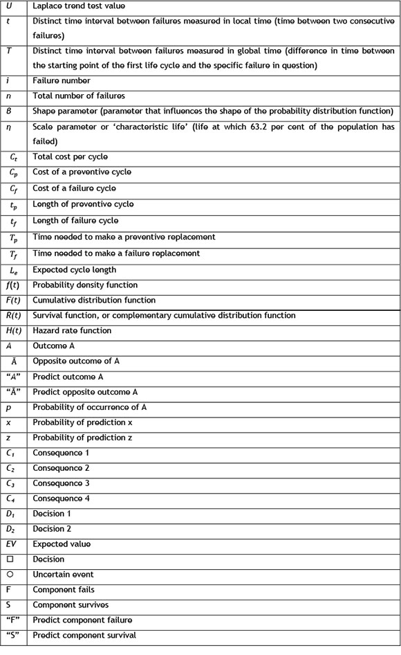
2 VARIABLES USED

In order to simplify the referencing of variables used in this paper, this section defines all the variables used.

 

 

3 LITERATURE

3.1 Decision-making in maintenance

Maintenance managers and practitioners are often confronted with difficult decisions related to the replacement and repair of physical assets, taking into account the cost, risk, and performance of the assets [1]. So various methodologies have been developed for dealing with such decisions - particularly the decision about which maintenance strategy or tactic should be used for each maintenance-significant item of the total system. Decision analysis is one method that can assist the maintenance manager in making rational decisions in optimising maintenance cost under conditions of uncertainty. In maintenance management uncertainty relates to the failure times of items, repair or replacement times, and lead time for spare parts, to name a few.

De Almeida and Bohoris [2] reviewed basic decision theory concepts and which steps could be applied in practice in the maintenance environment. They built a maintenance decision model and outlined its applicability in a case study of a power station. Backlund and Hannu [3] investigated the effect of different risk analyses approaches on the quality of maintenance decisions. These authors emphasised that risk analysis results should be analysed and interpreted carefully before making maintenance decisions.

Walls et al. [4] proposed a decision science methodology for evaluating alternative maintenance strategies. This method uses decision diagrams and the 'value of information' framework to analyse maintenance decisions by considering the mean-time-between-failure (MTBF) and the cost of replacement. Labib [5] developed a decision-making grid to assist in choosing a specific maintenance strategy. This method aims to establish a Pareto analysis of two important criteria: downtime and frequency of calls. Items are then mapped on a grid and a maintenance strategy is recommended based on their position on the map.

Pintelon et al. [6] identified two categories in maintenance management where decision theory could be applied: decisions in a risk environment, and decisions in an uncertain environment. Decisions in a risk environment can be used if sufficient data is available to define a probability density function. Decision-making for this situation usually involves the optimisation of the expected value (EV).

A naturalistic maintenance decision model is proposed by Grobbelaar and Visser [7]. This model suggests that maintenance decision-makers should use their intuition to select a maintenance strategy and then use analytical methods to confirm the accuracy of their decision. Many maintenance decisions require an analysis of several competing criteria. Triantaphyllou et al. [8] illustrate how the most important criteria can be determined for a multi-criteria decision-making application in maintenance.

3.2 Renewal theory

The application of renewal theory in maintenance and reliability management was introduced as early as 1939 [9]. This statistical method uses distribution functions - for example, the Weibull distribution function - to determine the optimal replacement intervals for components. Renewal theory assumes that replacement will take place directly after the failure has occurred, and that it can only be applied to non-repairable components that are discarded after their first failure [10,11]. Renewal theory is not applicable where the failure data indicates that the component's or system's reliability improves (failure rate decreases with each replacement) or deteriorates (failure rate increases with each replacement; typical of refurbished components) [10]. In these cases, repairable systems theory - for example, the non-homogeneous Poisson process model -should be used. This paper will be limited to failure data that can be modelled using renewal theory.

Various probability distributions, such as the normal, lognormal, Weibull, and gamma distributions, can be used to model the time-to-failure of components of a system. In this paper, only the Weibull probability density function is considered. In cases where a component is replaced before it has failed, or where it has failed subsequent to a failure of another component that is not under investigation, the data is considered to be suspended. In these cases, the ranks of the data have to be adjusted. The data of a Weibull plot should form a straight line, but in some cases it appears curved. This can occur for various reasons, and is likely because the life of the component will always be more than a specific period. In these cases it is more appropriate to use the three-parameter Weibull distribution function [12]. This paper will not consider suspensions (replacements that took place before a failure occurred or due to the failure of another component) and will only use the two-parameter Weibull distribution function. Although this paper presents the process that was followed to develop a model for determining the value of predictive maintenance for specific conditions, the same process can be used to develop models under different conditions - such as when the failure data requires that a different distribution function be used.

3.3 Laplace trend test

Since this paper is limited to failure data to which renewal theory can be applied, the first step is to determine whether renewal theory provides an appropriate model of the failure data. In order to determine this, the Laplace trend test is used. This test (also referred to as the centroid test) is used to determine whether there is a trend in the chronologically-ordered failure data. The test statistic, U, is calculated by means of Equation 1 [13]:

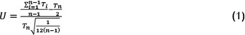
If 1 > U > -1, there is no underlying reliability degradation or improvement, and thus renewal theory can be applied [11].

3.4 Weibull probability density function

The Weibull probability density function provides the probability of failure of a component at a given time, and can be determined by means of Equation 2 [12]:

3.5 Determination of parameters of distributions

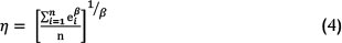
The parameters of a probability distribution (Weibull or other distribution) for a component can be determined from failure data, using various methods. One method is to use special probability graph paper. Failure times of the component are ordered and the cumulative probability of failure is estimated. This cumulative probability is plotted typically on the Y-axis of the probability paper, and the failure time is plotted on the X-axis. If a straight line can be fitted through the data points, the distribution selected is an appropriate model for the failure behaviour. The parameters can also be determined by iterative methods and by a least squares fit of the cumulative distribution function of the failure data. Using the maximum likelihood method, the shape (β) parameter of the Weibull distribution function can be determined iteratively from the following equation [12]:

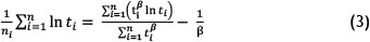
The value obtained for β can now be substituted in Equation 4 to obtain the value of the scale parameter (η) of the Weibull distribution [12].

The probability distribution function, reliability function, and determination of the parameters of the distribution are used to develop the equations for the determination of the EV of information for non-repairable components.

3.6 Optimal preventive replacement age of component

Preventive maintenance of a component has the obvious benefits of reducing downtime and causing no sequential damage to other components of a system. However, making replacements too frequently increases the cost; there is therefore an optimum replacement interval that will provide an optimum (minimum) cost of maintenance. The maintenance cost per unit time for preventive maintenance is given by Equation 5 [14]:

The optimal replacement cost per unit time will be where C(t_p) has the lowest value for a series of t_p. The specific value of t_pcan be determined either through graphical inspection or differentiating the equation for C(t_p), setting it equal to zero and solving for t_p[10].

3.7 Decision analysis

Basic decision analysis was developed as early as 1654 by Blaise Pascal and Pierre de Fermat, to calculate the probabilities of chance events [15]. The purpose of decision theory is to assist a decision-maker in making decisions. Clemen and Reilly [16] wrote the following to indicate how useful the decision analysis technique is when difficult decisions have to be taken in business and projects:

"Decision analysis provides structure and guidance for systematic thinking in difficult situations. However, it does not claim to recommend an alternative that must be blindly accepted."

Bunn [17] also emphasised that the goal of decision analysis is not to replace the intuition of the individual decision-maker, but rather to support the decision-maker in understanding the nature of a particular problem or situation. Raiffa [18] mentioned a common complaint about decision analysis: that it is often performed with imperfect input data. However, he added that it is better to make use of imperfect input data than using no input data at all.

The decision theory in the next section was adopted from Clemen and Reilly [16], and will indicate how the EV of imperfect information can be calculated by using decision trees.

3.7.1 Expected value (EV):

In order to determine the value of a chance event, the EV method is used. This method can also be used to determine the EV of predictive maintenance. The general EV method is discussed first and then combined with renewal theory to determine the EV of predictive maintenance. The EV is determined as the weighted average of the possible outcomes. Decision trees illustrate the probability of occurrences, possible outcomes, and consequences. Decision trees comprise decision- or action-nodes as well as event- or chance-nodes.

For a situation where there are two possible consequences resulting from an event, the problem can be illustrated through a probability tree, as shown in Figure 1 [16]:

 

 

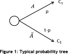
The EV is then given by Equation 6:

3.7.2 Expected value (EV) of information:

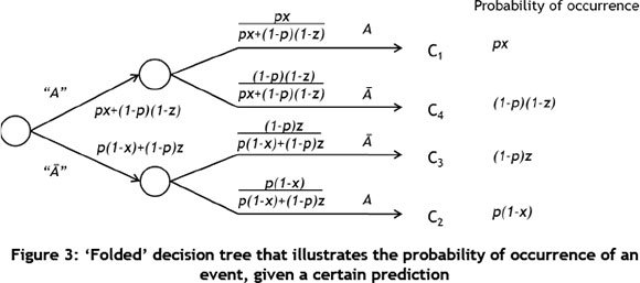
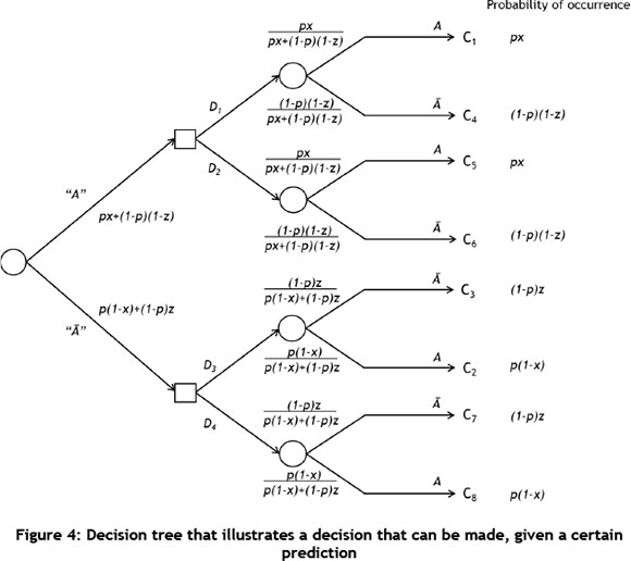
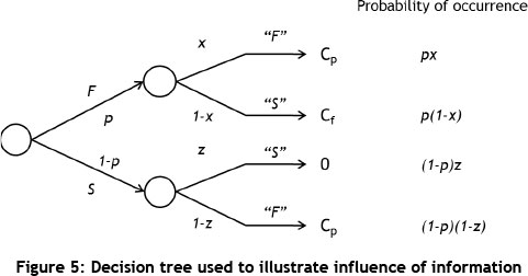
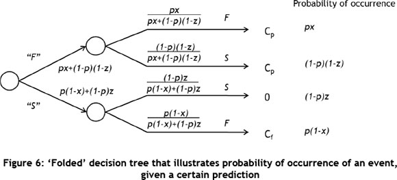
Decision trees can also be used to illustrate how information (prediction of a possible outcome) can be used to choose between alternatives. Decision can help to indicate what the probability of a specific outcome is, given that a decision was made subsequent to a prediction. This method can be used to determine the EV of information. For example, it can be used to determine the value of a weather forecaster, given that the weather on a particular day will have a monetary influence. To illustrate such a problem, the decision tree is first illustrated in the normal format, as indicated in Figure 2. The 'folded' tree is illustrated in Figure 3, and then decision positions are added to the diagram, as given in Figure 4. This process is generic, and is taken from Clemen and Reilly [16]. However, the exact application is problem-specific, and the decision tree example provided below is specifically for the application in this paper.

 

 

 

 

 

 

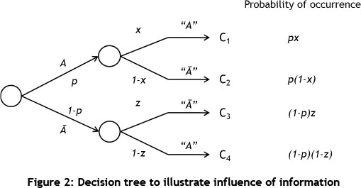
The EV for the decision tree in Figure 2 is given by the following equation:

The EV of information can be calculated by subtracting the EV subsequent to a prediction, from the EV without a prediction. In the case of the weather forecaster, the EV of information can be determined by subtracting the expected monetary value of a specific day without using a weather forecaster from the expected monetary value when a forecaster, whose forecasting accuracy is known, is used.

 

4 VALUE OF INFORMATION FOR NON-REPAIRABLE COMPONENTS

In many cases it can be more cost-effective to replace a component preventively rather than reactively, especially if a failure causes damage to other equipment. Following this, a component can be replaced preventively based either on the time it has been used (preventive maintenance) or on its condition (predictive maintenance). The assumption in predictive maintenance is that failure age can be predicted based on some sort of measureable event or gradual deterioration. Thus in order to implement predictive maintenance, the condition of an asset has to be determined. If the condition is not satisfactory, repair or replacement has to be implemented. This type of maintenance is referred to as condition-based maintenance (CBM). Examples of such models can be found in Kaiser and Gebraeel [19], Swanson [20], and Ming-Yi et al. [21]. The purpose of this paper is not to prove that such predictive models exist nor that they are reliable; this paper assumes simply that they do exist and that their reliability can be defined in terms of a constant probability. Different condition monitoring techniques can be used, such as vibration measurement, temperature measurement, and oil analysis. The results from the condition measurement, in combination with a predictive model, can then be used to predict when a component will fail and whether the component should be replaced or not. The benefit of using predictive maintenance as a preventive maintenance strategy is that a component can be replaced based on its condition, and ideally just before it fails.

However, determining the cost per unit time of predictive maintenance is an area that is reasonably unchartered in the maintenance literature. This means that it is difficult to determine the EV of predictive maintenance, and thus it is difficult to determine whether or not a specific method of predictive maintenance will be financially viable to implement. Since predictive maintenance is essentially a predictive exercise, the value of predictive maintenance can be determined by using the EV of information method as explained above, and replacing the probability of occurrence (p) with the probability of failure (in this case f(t)). The results of this argument are illustrated below.

4.1 Main assumptions

In order to simplify the development of the model for determining the EV of information for non-repairable components, the following assumptions were made:

1. The failure data can be presented by a two-parameter Weibull probability density function.

2. The user will take action according to the prediction made by a predictive maintenance model in combination with a CBM technique (in other words, if it is predicted that the component will fail, it will be replaced; however, if it is predicted that the component will survive, it will not be replaced). If this is not the case, the decision tree will have to be extended by another level. This scenario is possible to model, but it is outside the scope of this paper.

3. The prediction can be perfect or imperfect. If the prediction is perfect, the probability of a prediction given an occurrence will be 1. If the prediction is imperfect, the probability of a prediction given an occurrence will be between 0 and 1. The value of the probability of the prediction is determined by the reliability of the predictive maintenance model. For instance, if the model is only correct 50 per cent of the time, then the probability will be equal to 0.5.

4. The probability of a prediction given an occurrence will always remain constant (the reliability of the predictive maintenance model will always be the same).

5. If, based on the results of the CBM technique, the predictive maintenance model predicts that the component will not fail and the component is subsequently not replaced, the associated maintenance cost is 0.

In order to simplify referencing, the following variables will be modified as follows:

p probability of occurrence, F

z probability of prediction, "S"

x probability of prediction, "F"

4.2 Expected value (EV) of predictive maintenance

Decision trees are used to illustrate how the EV of information technique is used in combination with renewal theory to determine the EV of predictive maintenance. The first step in the process is to illustrate the prediction scenario at any given time in terms of the EV of information, as indicated in the previous section. This process is illustrated below.

 

 

 

 

At any given point in time, the EV will thus be:

The expected cycle length for the example above is:

To determine the replacement cost per unit time, the total EV must be divided by the expected cycle length, as illustrated by Equation 10:

and be simplified to:

Since the assumption of a Weibull probability density function was made, the probability of failure (p) can be replaced by the Weibull probability density function (f(t)). Thus at any given point in time:

Subsequently, the following equation can be derived to calculate the EV of preventive maintenance per unit time:

If replacement time is negligible compared with failure time, this can be simplified to:

To determine which maintenance strategy should be used, the difference between the EVs should be calculated. The maintenance strategy with the lowest cost is preferable. Most maintenance strategies cost money to implement. This cost can be added to the EV to calculate the total cost of the strategy. Again, the different strategies can be evaluated against each other to determine which strategy will be the most cost-effective to implement.

 

5 EXAMPLE

In order to illustrate how this model can assist with maintenance decision-making, a simple hypothetical example will be provided. Important to note is that the data was selected randomly, and that the aim is to illustrate the application of the process, and not to imply a preference for a specific maintenance strategy. In this example, the decision-maker will have to choose between implementing a run-to-failure, a preventive maintenance, or a predictive maintenance strategy.

5.1 Hypothetical problem

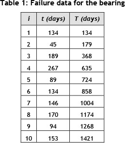
A maintenance practitioner has been contacted by a condition-monitoring consultant who argues that he/she can significantly reduce the maintenance costs of the maintenance practitioner's company by implementing predictive maintenance on an electrical fan motor that is used continuously for 350 days per annum. Based on historical data, the maintenance practitioner has determined that a specific bearing within the assembly (including the electrical motor and the fan) determines the lifetime of the assembly. Thus, if the bearing survives, the assembly survives. However, if the bearing fails, it leads to consequential damage and the whole assembly has to be replaced. The maintenance practitioner has gathered failure data on the bearing, illustrated in Table 1, where t is the failure time of the i^th failure and T is the cumulative value of the failure times.

 

 

Based on historical data, the maintenance practitioner has determined that if the bearing were replaced preventively, it would cost ZAR 650. However, if the bearing failed, the total replacement cost would amount to ZAR 60,000 (including replacement of the full assembly). The specific company uses 20 of these fan assemblies in similar conditions, for which the failure data is also similar. According to the CBM consultant, their predictive maintenance model will correctly predict 95 per cent of failures, and will never have give false alarms. The CBM consultant proposes to the maintenance practitioner that they can provide this predictive maintenance model (including the monitoring equipment) to their company at a total annual cost of ZAR 80,000.

The maintenance decision-maker decided that before the predictive maintenance strategy were implemented, it should be compared with other options. The maintenance decision-maker decided that four strategies should be considered:

• run-to-failure;
• preventive maintenance based on the MTBF;
• preventive maintenance based on the optimal preventive replacement age of the component; and
• predictive maintenance.

5.2 Assumptions

• the impact of stopping for 15 days of the year can be ignored;
• all occurrences are failures, i.e., no suspensions;
• all failures led to replacement of the complete assembly; and
• in order to calculate the preventive maintenance cost of replacement at the MTBF, the preventive replacement age was set to the MTBF (i.e., t_p = MTBF) and inserted into Equation 5.

5.3 Calculations

The first step was to determine whether renewal theory was applicable. In this case, U = -0.041 and thus renewal theory could be used.

Subsequently the Weibull shape and scale parameters can be estimated:

β = 2.63

η = 159.96

The following constants were used:

C_p= ZAR 650

C_f = ZAR 60,000 z = 1

x = 0.95

The constants can then be inserted into Equation 14:

This equation can then be simplified to:

Using numerical integration, the cost of the various maintenance strategies can be calculated as shown in Table 2.

 

 

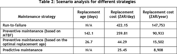
5.4 Recommendations

By implementing the predictive maintenance strategy, the total annual replacement cost saving for 20 fans is approximately ZAR 2,776,892. In this case, the predictive maintenance strategy should also be ZAR 131,882 per annum less than a preventive maintenance (based on the Weibull probability density function) strategy if implemented on all 20 fans. Thus at an annual fee of ZAR 80,000, the predictive maintenance strategy should be implemented.

 

6 CONCLUSIONS AND RECOMMENDATIONS

The benefit of CBM is that information about the condition of a component is available. With this information, in combination with a predictive maintenance model, a prediction can be made about whether a component will fail; subsequently it can be decided whether it should be replaced. This paper has illustrated how a model was developed to calculate the EV of information for non-repairable components that can be used to determine the replacement cost per unit time of a predictive maintenance strategy. This predicted cost can then be compared with the cost of alternative maintenance strategies, and thus be used to choose between maintenance strategies.

Future research should focus on case study analyses to determine the practical application of this model, as well as to expand the theory to repairable systems. By confirming the practicality of this model, and by expanding its application area, it should become a very useful tool for maintenance decision-makers to use when choosing between maintenance strategies.

 

REFERENCES

[1] International Organization for Standardization. 2014. ISO 55001, Asset management -Management systems - Requirements. Retrieved from http://www.iso.org/iso/catalogue_detail?csnumber=55089 (Accessed on 23 March 2015).         [ Links ]

[2] De Almeida, A.T. & Bohoris, G.A. 1995. Decision theory in maintenance decision making, Journal of Quality in Maintenance Engineering, 1(1), pp. 39-45.         [ Links ]

[3] Backlund, F. & Hannu. J. 2002. Can we make maintenance decisions on risk analysis results? Journal of Quality in Maintenance Engineering, 8 (1), pp. 77-91.         [ Links ]

[4] Walls, M.E., Thomas, M.E. and Brady, T.F. 1999. Improving system maintenance decision: A value of information framework, The Engineering Economist, 44(2), pp. 151-167.         [ Links ]

[5] Labib, A.W. 2004. A decision analysis model for maintenance policy selection using a CMMS, Journal of Quality in Maintenance Engineering, 10(3), pp. 191-202.         [ Links ]

[6] Pintelon, L.M., Gelders, L.F. & Van Puyvelde, F. 1997. Maintenance management. Belgium: Uitgeverij Acco.         [ Links ]

[7] Grobbelaar, S. & Visser, J.K. 2010. Evaluating strategic maintenance decision making, Conference Proceedings: Euromaintenance International Maintenance Conference. Verona, Italy, May 12-14, pp. 105-109.         [ Links ]

[8] Triantaphyllou, E., Kovalerchuk, B., Mann, L. & Knapp, G.M. 1997. Determining the most important criteria in maintenance decision making, Journal of Quality in Maintenance Engineering, 3(1) pp. 16-28.         [ Links ]

[9] Rueda, A. & Pawlak, M. 2004. Pioneers of the reliability theories of the past 50 years, Reliability and Maintainability Annual Symposium - RAMS, pp. 102-109.         [ Links ]

[10] Coetzee, J.L. 1997. Maintenance. Hatfield: Maintenance Publishers.         [ Links ]

[11] Vlok, P.J. 2012. Introduction to elementary statistical analysis of failure time data: long term cost optimization and residual life estimation. Published as part of the Quality Management 444 course presented at the Department of Industrial Engineering, University of Stellenbosch.         [ Links ]

[12] Evans, M., Hastings, N. & Peacock, B. 2000. Statistical distributions, 3^rd edition, New York: John Wiley & Sons.         [ Links ]

[13] O'Connor, P.D.T. 2008. Practical reliability engineering, 4^th edition, West Sussex, England: John Wiley & Sons, Ltd.         [ Links ]

[14] Jardine, A.K.S. 1973. Maintenance, replacement and reliability. New York, USA: Pitman Publishing.         [ Links ]

[15] Buchanan, L. & O'Connell, A. 2006. A brief history of decision making, Harvard Business Review, 84(1), pp. 32-41.         [ Links ]

[16] Clemen, R.T. & Reilly, T. 2001. Making hard decisions with decision tools, USA: Duxbury.         [ Links ]

[17] Bunn, D. 1984. Applied decision analysis, New York: McGraw-Hill.         [ Links ]

[18] Raiffa, H. 2002. Decision analysis: A personal account of how it got started and evolved, Operations Research, 50(1), pp. 179-185.         [ Links ]

[19] Kaiser, K.A. and Gebraeel, N.Z. 2009. Predictive maintenance management using sensor-based degradation models, IEEE Transactions on Systems, Man and Cybernetics, Part A: Systems and Humans, 39(4), pp. 840-849.         [ Links ]

[20] Swanson, D.C. 2001. A general prognostic tracking algorithm for predictive maintenance, IEEE Proceedings from the Aerospace Conference, 6, pp. 2971-2977.         [ Links ]

[21] Ming-Yi, Y., Lin, L., Guang, M. & Jun, N. 2010. Cost-effective updated sequential predictive maintenance policy of continuously monitored degrading systems, IEEE Transactions on Automation Science and Engineering, 7(2), pp. 257-265.         [ Links ]

 

 

* Corresponding author
¹ The author was enrolled for the M Eng (Technology Management) degree in the Department of Engineering and Technology Management, University of Pretoria