GENERAL ARTICLES

 

Selection of a decision model for rolling stock maintenance scheduling

 

 

O.O. Asekun; C.J. Fourie

Department of Industrial Engineering University of Stellenbosch, South Africa. cjf@sun.ac.za

 

 

---

ABSTRACT

Rolling stock is the most maintenance intensive part of the railway system and therefore, the most vulnerable if maintenance is neglected. It is therefore, essential to have an efficient maintenance schedule for rolling stock components. A decision support model can be used to achieve this. However, selecting the appropriate model to achieve this is vital to the success of the decision support model. In this paper a practical way of selecting the appropriate model to develop a decision support for scheduling of rolling stock maintenance, is presented. A case study is used as a numerical example for the proposed framework.

---

OPSOMMING

Die rollende voorraad van 'n spoorwegstelsel vereis gewoonlik intensiewe instandhouding en daarom is dit die meeste kwesbaar indien instandhouding afgeskeep word. Dit is dus noodsaaklik dat 'n doeltreffende instandhoudingskedule vir rollende voorraad onderdele gebruik word. Om dit moontlik te maak, kan 'n besluitsteunmodel gebruik word. Om 'n suksesvolle besluitsteunmodel daar te stel, is dit egter noodsaaklik om die mees geskikte model hiervoor te kies. In hierdie artikel word 'n praktiese metode voorgestel om die mees geskikte model te kies vir die ontwikkeling van 'n skedulering besluitsteunmodel.

---

 

 

1 INTRODUCTION

Rolling stock assets are capital intensive in rail companies, therefore if a railway service is to be reliable, the equipment must be kept in good working order. This means that an efficient maintenance schedule is an essential factor to achieving a reliable rolling stock system. Railway systems consist of both mechanical and electrical components combined into several systems containing a large number of moving parts. To achieve an acceptable railway service level, each system needs to kept operational and regular maintenance is the essential factor to achieving this. A railway system can be sub-divided into two sub-systems namely: rolling stock and Infrastructure. Rolling stock refers to all the vehicles that move on a railway. These vehicles can either be powered or unpowered vehicles or a combination of both, some example of rolling stock include locomotives, railroad cars, coaches and wagons. Rolling stock is the most maintenance intensive part of the railway system and therefore, the most vulnerable if maintenance is neglected. The importance of the maintenance functions and maintenance management has greatly grown in all sectors of manufacturing and service organizations. The principal reason for this growth is the continuous expansion in the capital inventory, the requirements for the functioning of systems and the outsourcing of maintenance.

When modelling the reliability of systems, there is a general assumption that failures of components are identical and independently distributed. This assumption is not necessarily always true and as a result wrong analysis and results are achieved in most cases. This article proposes a framework for selecting the appropriate model for rolling stock components. The rest of this paper is organized as follows. Section 2 presents a brief literature review on rolling stock maintenance and maintenance decision models and classification of these models. Section 3 shows a description of non-repairable and repairable systems, collection of failure data and methods used to test for trends are explained in this section. The models applicable to the results of the trend are also presented in this section. Section 4 shows the procedure to select an appropriate model for rolling stock maintenance scheduling. Section 5 presents data from a case study which is analysed using the proposed selection procedure. Section 6 highlights the concluding remarks and summary of findings of the research carried out in this paper.

 

2 LITERATURE REVIEW

2.1 Rolling stock maintenance

Railway industries have been considered as an environmental friendly transportation mode and its demand has been increasing over the years. There is a need to maintain a high level of reliability, safety, availability and maintainability within a rail system. This however, is a challenging task to accomplish considering the two main sub-systems that make up the railway system, namely the rolling stock and infrastructure. Infrastructure includes signal, power supply and rail tracks while Rolling stock refers to all vehicles that move on a rail track which could be coaches, wagons and locomotives. Of these two, Rolling stock can be classified as the most important and most vulnerable [1].

Rolling stock has a huge effect on the service level of the system because the service level of the rail system is directly proportional to the safety and comfort of the passengers. In order to achieve the required service level, the quality of the rolling stock performance needs to be improved continually and this can be achieved with proper maintenance. A train is also classified as rolling stock and it comprises of several rail vehicles connected in series. The combination of these vehicles are complex, but can be redistributed and reconfigured to include embedded systems, which are combined together to provide a high quality transportation service [2].

Rolling stock maintenance has been categorized generally into Corrective maintenance (CM) and preventive maintenance [3]. Nevertheless, these maintenance strategies have been found to be ineffective. Majority of maintenance activities in rolling stock companies are directed towards preventive maintenance, which often leads to incorrect maintenance work, frequent down time, unnecessary maintenance tasks and often reverts to CM or breakdown maintenance [4]. Given this scenario, rolling stock industries need to be able to manage these strategies effectively by creating efficient schedules to perform the selected maintenance strategy.

2.2 Maintenance decision models

Since maintenance became a frequent practice of industries, researchers have worked on various ways to efficiently schedule maintenance. The maintenance scheduling problem can also be formulated as a maintenance optimization problem [5]. The aim would be to find an optimum balance between maintenance cost and maintenance objectives while considering all possible constraints. For example, the aim can be to derive a solution to either minimize or maximize system maintenance cost and a maintenance objective such as system reliability measures or some sort of other performance indicator. It could also be a combination of the two criteria to minimize maintenance cost and maximize reliability simultaneously [6].

Maintenance optimization models in this paper are defined as those models or processes by which maintenance strategies, planning or scheduling is being improved. Maintenance optimization models are made up of mathematical models which focus on deriving the optimal balance between maintenance costs and benefits of maintenance or the most appropriate time to execute maintenance. Several factors are considered when attempting to achieve an optimal maintenance schedule. These factors include: safety, health, environment, maintenance cost, failure cost, opportunity cost and replacement cost [7].

2.3 Classification of maintenance optimization

Maintenance optimization models can either be qualitative or quantitative. Qualitative models include TPM, RCM, and plant asset management (PAM) while quantitative models include deterministic/stochastic models such as Markov decision, Bayesian models and integer programming It is important to note that maintenance optimization is only a tool to improve the overall maintenance process and therefore, to achieve an effective performance in the maintenance process, the optimization model, maintenance policies, maintenance costs and system reliability all need to be considered instantaneously [6]. A general model for maintenance optimization is presented in Vatn [8] where safety, health and environmental objectives, maintenance costs, downtime cost are all taking into consideration.

Maintenance optimization can be classified using the objective, planning horizon, decision factors and the number of components of the problem [9]. The different classification of maintenance optimization is presented in Table i.

 

 

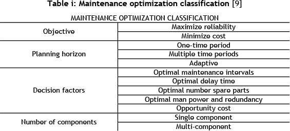
Considering the classifications of optimization discussed above, rolling stock maintenance problems can be modelled as multi-component optimization problems in that a rolling stock system for example a train is made of motor coaches and trailers connected in series. The motor coaches and trailers consist of both reparable and non-repairable systems. Optimization of multi-component systems has been reported in literature to an extent [10], [11], [12].

 

3 NON-REPAIRABLE AND REPAIRABLE SYSTEMS

Engineering systems can either be repairable or non-reparable. Non-repairable systems refer to systems in which when a failure occurs, the system is discarded because repairing the system is not economically feasible. Examples of these systems include electric bulbs, missiles and non-degradable batteries. In these systems, the reliability of the systems is required to be high and is modelled using statistical distributions such as Weibull. Repairable systems refer to systems that go through many phases of failure and repair within the duration of their design life. The reliability of these systems does not generally have to be as high as that of non-repairable systems. Reliability of repairable systems is modelled by using stochastic point process [13].

Louit [13] discussed five main stochastic process models than can be applied to modelling a repairable system namely the renewal process (RP), the homogeneous Poisson process (HPP), the branching Poisson process (BPP), the superposed renewal process (SRP) and the non-homogeneous Poisson process (NHPP). Of these five, the two widely used stochastic process models applied to modelling repairable systems in literature are the Homogeneous Poisson process (HPP) and the Non-Homogeneous Poisson process (NHPP). A method of improving repairable systems is making use of highly reliable components for the system and applying an efficient repair or maintenance system. The two most important performance criteria for repairable system are reliability and inter-arrival failure times [14]. In fitting a repairable system into a distribution, it is assumed that the failures are always statistically independent and identically distributed, although this may not always be the case. When a component failure occurs in a repairable system, the remaining components have a current age. Therefore, the next failure of the component depends on its current age. Thus, the failure events at the system level are dependent. This property forms an important characteristic of a repairable system. If the times between sequential failures are increasing, then the reliability of the system is improving. If the times between sequential failures are decreasing, then the systems' reliability is degrading.

3.1 Failure data

Gathering the right information for reliability improvement is a very crucial and important aspect of reliability analysis. However, this process is faced with different challenges and limitations. One of the common challenges in reliability analysis is lack of adequate data to carry out proper statistical analysis. As pointed out by Louit [13] the amount of data available places a limit on the capabilities of statistical methodologies used for analysis. It is believed that this problem would never disappear given that the aim of maintenance is to reduce failure occurrence. Another practice during data collection is data censoring. Censored data refers to stopping a collection of data when the unit has not failed and the exact failure time in not known. It can either be left, interval or right censored [15].

3.2 Trend test methods

In analysing a repairable system, it is important to determine if there is a trend in the data set that has been gathered by analysing the changes of inter-arrival failures occurring over a certain period of time of the system. The results of this test can be used to model the system to follow either the HPP or NHPP. A system can have various monotonic or nonmonotonic trends; monotonic trends means there could be reliability growth which implies times between failures are occurring longer with time. It could also be reliability degradation, which means times between failures are decreasing with time. Non-monotonic such as cyclic, bathtub curves could also be present. Statistical hypothesis test is an effective way to check inter-arrival failure times for a trend [16]. Such tests include Graphical methods, Laplace, Lewis Robinson trend test and the Military handbook test.

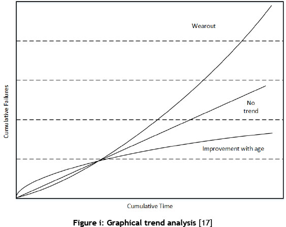
3.2.1 Graphical methods

Graphical methods can be used to show if there is a trend in the rate of occurrence of failures, the simplest graphical method is achieved by plotting the cumulative failures against cumulative operating time. If no trend is found in the data, a line fitted through the data will be a straight line. A convex curve indicates an increasing failure trend; a concave curve indicates improvement with age [17]. These possibilities are shown in Figure i. Other graphical methods include scatter plot of successive service lives, Nelson-Aalen plot, Total time on test plot [13][18].

 

3.2.2 Laplace Test

This test is used to test a set of data for the null hypothesis of HPP against the alternative of NHPP. The test statistic under the null hypothesis is approximately a standard normal distribution variable. The Hypothesis test as presented by [l9] is:

Under H₀and conditioning on T₁,T₂,... ... . .,T_nare uniformly distributed, the test statistic for a time censored data is

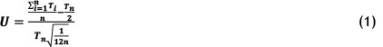
Where:

T_i is the time from a given start point to the time of each failure event

T_n is end time of the observation period

η is the number of failures

For time uncensored data, η is replaced with η - 1 and T_n by τ

The rejection criteria are based on the standard normal distribution assumption for U. This is given by:

Reject H₀if U > Za_/2or U < -Za_/2. at 95% confidence interval.

According to [18], rejecting H₀only confirms that the data does not follow HPP. It does not necessarily imply that there exist a trend in the data hence a need to apply a renewal trend test to check if the data follows a trend.

3.2.3 The Military handbook test(MHB)

This is similar to the Laplace test because the null hypothesis is to check for HPP against NHPP. This measure under the null hypothesis is χ²distributed with 2ndegrees of freedom under the null hypothesis and is defined as:

H₀: HPP

H_a: NHPP

Under H₀and conditioning on T₁, T₂,... ... . . ., T_nare uniformly distributed, the test statistic for a time censored data is

Where T_t, T_nand η have the same meaning as in the Laplace test.

For time uncensored data, η is replaced with n- 1 and T_nby τ

The rejection criteria are based on the chi-square distribution with 2 degrees of freedom assumption for . This is given by,

Reject H₀if ΜΗ > χ²_aat 95 percentile or ΜΗ < χ²_aat 5 percentile

3.2.4 Lewis-Robinson test

The Lewis-Robinson (LR) test is a modification of the Laplace test that tests the data for a null hypothesis of a renewal process (RP) using the failure inter-arrival failure times [18]. The Hypothesis test as presented by [19]is

H₀:RP

H_a: Not RP

The LR test statistic is derived by dividing the Laplace statistic by the coefficient of variation ( CV) for the observed inter-arrival failure times.

where CV is derived as the variance of X divided by the Mean of X

where X is the inter-arrival times variable.

The rejection criterion is similar to that of Laplace. Which is given by, Reject H₀if LR > Za_/2or LR < -Za_/2. at 95% confidence interval

3.3 Homogeneous Poisson Process (HPP)

If we have a counting process N(t) >, t > 0 that represents a total number of events (failure or repairs) that have occurred up to time , the counting process ( ) must satisfy the following conditions for an HPP process [15]:

1. (t) > 0

2. (t) is an integer value

3. [ N(t),t > 0] has independent iηcrements. i.e N(t₂) - N(t₁) 1 N(t₁)

4. if t₁ < t₂, then N(t₁)< N(t₂), and

5. The number of events that occur in the interval [t_1,t2] where t₁<t₂is N(t₂) -N(t₁). The 5^th condition for HPP is modified in such a way that the number of failure events in the interval [t_1,t2] has a Poisson distribution with mean λ(t₂- t₁) where λ is the failure rate with condition (0) = 0.

Therefore, the probability of having η failures in the interval [t₁, t₂] is:

This follows that the expected number of failures in [t₁, t₂] is:

The reliability function of the HPP for the interval [t_lt t₂] is

A very good example of a HPP model is the Weibull model.

3.4 Non- Homogeneous Poisson Process (NHPP)

Analysing a repairable system by applying a distribution analysis may not be suitable for an effective analysis of a repairable system considering the characteristics of its failure events. For this reason, a stochastic process such as the Non-Homogeneous Poison Process (NHPP) would be suitable for such analysis. The NHPP has been proven by literature to be a suitable model for data that have trend. NHPP models are mathematically straightforward and their theoretical base is well developed. The model has been tested and vastly applied in literature [20]. The NHPP signifies that the failure intensity function is not time dependent. A NHPP must satisfy the following conditions [14]:

1. N(t) > 0

2. N(t) is an integer value

3. [N(t),t > 0] has independent increments. i.e N(t₂) - N(t₁) N(t₁)

4. if t₁ < t₂, theη N(t₁ < N(t₂), and

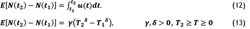
5. The number of events that occur in the interval [t_l,t2] where t₁ < t₂has a Poisson distribution with mean u(t) dt.

Therefore, the probability of having η failures in the interval [t₁, t₂] is

The expected number of failures in [t_lt t₂] is:

The reliability function of the NHPP for the interval [t₁ t₂] is

There are two methods in literature for applying the NHPP for repairable systems, namely the power law intensity and the log linear intensity. [21], [22], [23], [19] & [24].

3.4.1 Power law NHPP

The power law NHPP is given by

Where

u(t) is the failure intensity. I.e. Rate of occurrence of failure

γ is the scale parameter (failure function)

δ is the shape parameter(improvement/degradation)

The parameter δ can be used to understand the reliability growth of the system. δ < 1 implies that there's reliability growth and δ > 1 implies that there is reliability degradation.

From the definition of NHHP, the expected number of failures for the interval t_1t t₂ is

The reliability function for the interval t_1t t₂is given by

3.4.2 Log Linear NHPP

The log linear NHPP is given by

This format of NHPP gives a good representation of a repairable system with a₁ > 0. Similarly, from the definition of NHHP, the expected number of failures for the interval t_l, t₂ is:

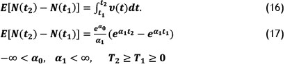
The reliability function for the interval t₁, t₂ is given by

3.5 Parameter Estimation

Parameters of NHPP can be estimated by using either the maximum likelihood method (MLE) or the least-square method. MLE method is a process that involves maximising the log likelihood of the power law function given by,

Such that,

Such that

The least square method involves minimizing the difference between the observed number of failures and the expected number of failures using the following function for the power law NHPP

For log linear NHPP

The least square method is a preferable parameter estimation method because it leads to more appropriate parameters than the MLE [21].

Reliability prediction is an area in literature that has gained much argument and attention; Reliability is not a parameter that is easily predictable on the basis of the laws of nature or of statistical analysis of past data. It is important to note that when forecasting reliability, any change in the physical system or in the change of operations will alter the prediction outcomes. It is therefore important to appreciate that the predictions of reliability can seldom be considered as better than rough estimates and that the achieved reliability can be considerably different to the predicted value [25].

 

4 MODEL SELECTION

Several authors have discussed methods by which a model should be selected for maintenance analysis [3], [5], [10]. To select an appropriate model for rolling stock maintenance, the discussed analysis should be performed by carrying out the following steps:

1. Select components: The first step is to define the components to be modelled and identify similar systems with the components.

2. FMMS: The next step is to gather the failure data of the component(s) to be modelled from the maintenance database. The time to each failure is recorded for the observation period; these times are arranged in chronological order.

3. Trend testing: This is to test the data for a trend. Any of the trend tests discussed can be applied to test for either a renewal process, HPP or NHPP. If no trend is found in the data, this means the data are independent and identical distributed and an HPP can be applied. On the other hand, if a trend is found in the data set, the data is assumed not to be independent and identical distributed and therefore a NHPP should be applied. If the trend results leads to a RP, this means the data are independent and identical distributed generated by a renewal process. The data should therefore be modelled by fitting a suitable statistical distribution like Weibull.

4. Intensity function: for NHPP, the intensity functions should be determined using the methods discussed in 3.4. The parameters estimated are used for the analysis of the rolling stock system.

This process is shown in the framework presented in Figure ii.

 

5 CASE STUDY

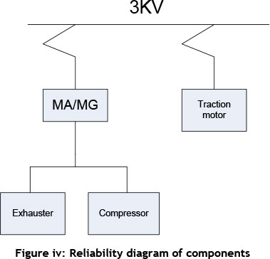
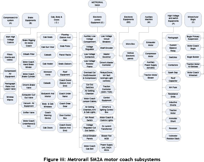
A numerical example to show the application if the selection step discussed above is presented. A few components of a 5M2A motor coach of Metrorail fleet at the Salt River Depot in Cape Town are selected. Figure iii shows the grouping of components of a 5M2A motor coach. An analysis performed shows that the traction motor and the auxiliary machines have the most occurrences of failures and therefore these components are selected for the numerical example.

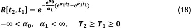
The data gathered from the fleet maintenance management system (FMMS) would consist of failure times of the following components, MA/MG, exhausters, compressor and traction motors between 2003 and 2013. Table ii shows the data set for the numerical example. This reliability block diagram of this components is shown in Figure iv, for the purpose of this example, We will consider the components are all connected in series because if any of these component fails, the reliability of the set is affected and the train set will stop.

 

 

 

 

5.1 Graphical Method

By plotting the cumulative failures versus time, we get four different plots for each of the components shown in Figure v to Figure viii.

 

 

 

 

 

 

 

 

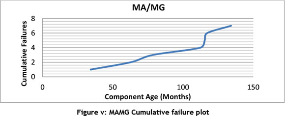
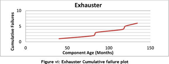
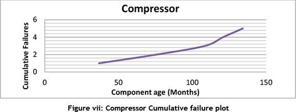
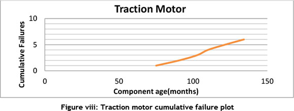
Comparing this plots with Figure i, it is uncertain what the trend in the data set is therefore performing a trend test that would be useful to ascertain the trend of the failure data to enable a right choice of model to analyse the reliability of the components. Table iii shows the result of performing the different trend tests discussed in 3.2.

 

 

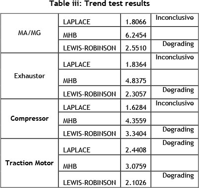
The results show that there is a trend in each of the data set and therefore the NHHP models for repairable systems should be applied.

 

6 CONCLUSION

This study reviews the process to undertake when selecting an appropriate model for rolling stock maintenance. It was established that a rolling stock is a multi-component system and each component should be analysed for reliability characteristics. The process helps to decide an appropriate model such as NHPP power law or log linear than the commonly used Weibull distribution for repairable systems. Numerical example was presented using some components of rolling stock, the results of the analysis of the components show that the components follow a NHPP model and therefore be modelled using NHPP repairable theory.

 

REFERENCES

[1] Park, G., Yun, W. Y., Han, Y. and Kim, J. 2011. Optimal preventive maintenance intervals of a rolling stock system, Quality, Reliability, Risk, Maintenance, and Safety Engineering (ICQR2MSE), 2011 International Conference on, IEEE, pp 427-430.         [ Links ]

[2] Umiliacchi, P., Lane, D., Romano, F. and SpA, A. 2011. Predictive maintenance of railway subsystems using an Ontology based modelling approach, Proceedings of 9th world Conference on Railway Research, May, pp 22-26.         [ Links ]

[3] Cheng, Y., Tsao, H. 2010. Rolling stock maintenance strategy selection, spares parts' estimation, and replacements' interval calculation, Int J Prod Econ, 128(1), pp 404-412.         [ Links ]

[4] Rezvanizaniani, S., Valibeigloo, M., Asghari, M., Barabady, J. and Kumar, U. 2008. Reliability centered maintenance for rolling stock: A case study in coaches' wheel sets of passenger trains of Iranian railway, Industrial Engineering and Engineering Management, 2008. IEEM 2008. IEEE International Conference on, IEEE, pp 516-520.         [ Links ]

[5] Paz, N. M., Leigh, W. 1994. Maintenance scheduling: issues, results and research needs, International Journal of Operations & Production Management, 14(8), pp 47-69.         [ Links ]

[6] Sharma, A., Yadava, G., Deshmukh, S. 2011. A literature review and future perspectives on maintenance optimization, Journal of Quality in Maintenance Engineering, 17(1), pp 5-25.         [ Links ]

[7] Dekker, R., Scarf, P. A. 1998. On the impact of optimisation models in maintenance decision making: the state of the art, Reliab Eng Syst Saf, 60(2), pp 111-119.         [ Links ]

[8] Vatn, J., Hokstad, P., Bodsberg, L. 1996. An overall model for maintenance optimization, Reliab Eng Syst Saf, 51(3), pp 241-257.         [ Links ]

[9] Hilber, P. 2008. Maintenance optimization for power distribution systems, Stockholm:KTH, pp 516        [ Links ]

[10] Laggoune, R., Chateauneuf, A., Aissani, D. 2009. Opportunistic policy for optimal preventive maintenance of a multi-component system in continuous operating units, Comput Chem Eng, 33(9), pp 1499-1510.         [ Links ]

[11] Chareonsuk, C., Nagarur, N., Tabucanon, M. T. 1997. A multicriteria approach to the selection of preventive maintenance intervals, Int J Prod Econ, 49(1), pp 55-64.         [ Links ]

[12] Moghaddam, K. S., Usher, J. S. 2011. A new multi-objective optimization model for preventive maintenance and replacement scheduling of multi-component systems, Engineering Optimization, 43(7), pp 701-719.         [ Links ]

[13] Louit, D. M., Pascual, R., Jardine, A. K. 2009. A practical procedure for the selection of time-to-failure models based on the assessment of trends in maintenance data, Reliab Eng Syst Saf, 94(10), pp 1618-1628.         [ Links ]

[14] Elsayed, E. A. 2012. Reliability engineering, Wiley Publishing.         [ Links ]

[15] Hamada, M. S., Wilson, A., Reese, C. S., Martz, H. 2008. Bayesian Reliability, Springer.         [ Links ]

[16] Ionescu, D. C., Limnios, N. 1999. Statistical and probabilistic models in reliability, Birkhauser.         [ Links ]

[17] Pecht, M. 2010. product reliability, maintainability, and supportability handbook, Second Edition, CRC Press.         [ Links ]

[18] Lindqvist, B. H. 2006. On the statistical modeling and analysis of repairable systems, Statistical science, 21(4), pp 532-551.         [ Links ]

[19] Coit, D. W. and Wang, P. :. 2005. Repairable systems reliability trend tests and evaluation, Proceedings of Reliability and Maintainability Symposium,         [ Links ].

[20] Coetzee, J. L. 1997. The role of NHPP models in the practical analysis of maintenance failure data, Reliab Eng Syst Saf, 56(2), pp 161-168.         [ Links ]

[21] Vlok, P. J. 2013. Introduction to elementary statistical analysis of failure time dat: Lomg term cost optimization and residual life estimation, Class Note, Stellenbosch.         [ Links ]

[22] Rigdon, S. E., Basu, A. P. 1989. The power law process: a model for the reliability of repairable systems, Journal of Quality Technology, 21(4),         [ Links ].

[23] Ascher, H., Feingold, H. 1984. Repairable systems reliability: Modelling, inference, misconceptions and their causes, Lecture Notes in Statistics, 7.         [ Links ]

[24] Krivtsov, V. V. 2007. Practical extensions to NHPP application in repairable system reliability analysis, Reliab Eng Syst Saf, 92(5), pp 560-562.         [ Links ]

[25] O'Connor, P., Kleyner, A. 2011. Practical reliability engineering, Wiley.         [ Links ]

 

 

* Corresponding author
** The author was enrolled for an M Eng. (Engineering Management) degree in the Department of Industrial Engineering, University of Stellenbosch.