CASE STUDIES

 

Studies in Swarm Intelligence techniques for annual crop planning problem in a new irrigation scheme

 

 

Sivashan Chetty^I ; Aderemi O. Adewumi^II

^ISchool of Mathematics, Statistics and Computer Science. University of Kwa-Zulu Natal. University Road, Westville. Private Bag X 54001, Durban, 4000, South Africa. mervinthree@gmail.com
^IISchool of Mathematics, Statistics and Computer Science. University of Kwa-Zulu Natal. University Road, Westville. Private Bag X 54001, Durban, 4000, South Africa. adewumia@ukzn.ac.za

 

 

---

ABSTRACT

Annual crop planning (ACP) is an NP-Hard type optimisation problem in agricultural planning. It involves finding optimal solutions for the seasonal allocations of a limited amount of agricultural land among the various competing crops that need to be grown on it. This study investigates the effectiveness of employing three relatively new Swarm Intelligence (SI) techniques in determining solutions to an ACP problem at a new irrigation scheme. The SI metaheuristics studied include Cuckoo Search (CS), Firefly Algorithm (FA), and Glow-worm Swarm Optimisation (GSO). The solutions determined by these SI techniques are compared against the solutions of Genetic Algorithm (GA), another population-based metaheuristic technique. This helps to determine the relative merits of the solutions found by the SI techniques. The results show that the SI algorithms delivered solutions superior to those of GA in determining solutions to the ACP problem at a new irrigation scheme.

---

OPSOMMING

Jaarlikse oesbeplanning is 'n NP-Hard soort optimiseringsprobleem in landbou beplanning. Dit behels die bepaal van optimale oplossing vir die seisoenale toekenning van 'n beperkte hoeveelheid landbougrond aan die verskeie mededingende gewasse. Hierdie artikel ondersoek die doeltreffendheid van drie relatiewe nuwe Swerm Intelligensie tegnieke om oplossings tot oesbeplanning by 'n nuwe besproeiingskema te vind. Die Swem Intelligensie tegnieke wat ondersoek is, is die Koekoek Soekmetode, die Vuurvliegie Algoritme en die Gloei-wurm Swerm Optimisering tegnieke. Die oplossings deur hierdie tegnieke verkry is vergelyk met dié verkry met die tradisionele Genetiese Algoritme. Dié vergelyking help om die relatiewe voordele van die nuwe Swerm Intelligensie tegnieke te bepaal. Die resultate toon dat die voorgestelde tegnieke beter oplossings as die tradisionele Genetiese Algoritme benadering gelewer het.

---

 

 

1 INTRODUCTION

Increases in population growth have increased the need for more food to be produced worldwide. At present, shortages in food supply have brought the hard-felt reality of starvation to the lives of millions of people. This is particularly true in 'fourth world' countries. To combat this problem in the future, the productivity of food must increase. The agricultural sector is the primary supplier of food in the world [1]. To try to meet the growing demand for food, the agricultural sector must increase its output. Optimising the production of food with current agricultural practices is important, but it is not enough to meet the future demands. To produce more food in the future, more land must be made available for agricultural production.

The allocation of land for agricultural production will depend on the decisions made by local authorities. For land to be allocated, it must be assessed to determine its suitability for agricultural production, and whether the crops grown on it will be sustainable in the future. This is important for economic development. To determine the agricultural potential of a given area of land, several factors must be considered. The main factors are soil characteristics and climate conditions [2]. For crop production, these factors will determine the types of crops that will most suitably adapt to the given environmental conditions. Other important factors are, among others, the natural land resources and agricultural trends.

Natural land resources such as lakes and rivers are very valuable commodities. They can be used to source irrigated water which, with rainfall, is important in determining the full agricultural potential of a given area of agricultural land. The agricultural trends will determine the types of crops that will bring the most suitable economic benefits.

When an area of land is allocated to develop a new irrigation scheme, and it has been finalised which crops will be cultivated, then solutions must be found to the hectare allocations among the competing crops. In determining the hectare allocations, it must be considered that different types of crops grow in different seasons, grow for different lengths of time, and have different plant requirements. These factors must be considered in order to determine feasible solutions.

The problem of trying to optimise the seasonal hectare allocations of a given area of agricultural land among the various competing crops that must be grown within a year is an NP-Hard type optimisation problem in agricultural planning, called 'annual crop planning' (ACP). ACP aims to determine solutions that will maximise the total gross profits earned from a given area of agricultural land, by making the most efficient use of the limited resources available for agricultural production. Limited resources include land, irrigated water supply, and the various costs associated with agricultural production. The solutions must satisfy the multiple land and irrigation water allocation constraints that are associated with ACP, in order to be feasible.

This research introduces a new ACP mathematical model, formulated by the authors of this paper, and intended to determine solutions to the ACP problem at a new irrigation scheme. Previous studies in crop and irrigation planning have used both single and multi-objective mathematical models. Many optimisation techniques have been used to provide solutions to these models. These include Linear Programming (LP), Simulated Annealing (SA), Particle Swarm Optimisation (PSO) and Evolutionary Algorithms (EAs), among others. Pant et al. [3] employed the Differential Evolution (DE) algorithm to provide solutions to a crop planning problem under adequate, normal and limited irrigated water supply. The objective was to maximise the net benefits gained, under these conditions. It was found that DE performed better than the programming tool LINGO. In [4], Pant et al. investigated the performances of four EAs in providing solutions to a crop planning problem. These algorithms included the Genetic Algorithm (GA), PSO, DE, and Evolutionary Programming (EP). Solutions were also determined using LINGO. The solutions showed that, of all the heuristic algorithms, GA performed poorly, and that DE, PSO, and EP were all comparable. Georgiou and Papamichail [5] used SA in combination with the Stochastic Gradient Descent Algorithm to determine solutions for the optimised water release policies of a reservoir. The released water had to be allocated efficiently among the various crops being grown. To maximise profits, the 'optimal' cropping pattern had to be determined. Wardlaw and Bhaktikul [6] used GA to solve a problem of irrigated water scheduling, using a 0-1 approach. The research found that GA performed well in being able to distribute irrigated water to several farm plots to satisfy the soil moisture content levels under water scarce conditions. The water allocations were done on a rotational basis. Sarker and Ray [7] proposed an improved EA known as the Multi-objective Constrained Algorithm (MCA), which was used to provide solutions to a multi-objective crop planning problem. The research found that MCA performed relatively better than the two other optimisation techniques used. These techniques included the ε-constrained method and the Non-dominated Sorting Genetic Algorithm (NSGAII). Raju and Kumar [8] compared the performances of GA and LP in providing solutions to a crop planning problem. The objective was to maximise the net benefits. The performances of GA and LP were relatively close. It was concluded that GA is an effective heuristic algorithm that can be used for irrigation planning. Reddy and Kumar [9] studied the effectiveness of using Elitism-Mutation Particle Swarm Optimisation (EMPSO) in determining the short-term release policies of irrigated water from a reservoir under water scarce conditions. The study concluded that the heuristic algorithm is effective in providing short-term solutions for multi-crop irrigation.

The objective of this paper was to investigate and compare the performances of three relatively new Swarm Intelligence (SI) metaheuristic algorithms, in determining solutions to an ACP problem at a new irrigation scheme. The algorithms investigated are Cuckoo Search (CS), Firefly Algorithm (FA) and Glow-worm Swarm Optimisation (GSO). To determine the relative merits of the solutions provided by these SI algorithms, their solutions have been compared against the solutions of a traditional population based metaheuristic algorithm, the Genetic Algorithm (GA). The solutions determined and comparisons made will indicate the possible strengths and/or weaknesses of the SI algorithms, in determining solutions to this ACP problem. The solutions found will be valuable in making suggestions concerning the seasonal hectare allocations for the crops that are required to be grown. To the best of our knowledge, the authors of this paper have not come across any other research that has used SI metaheuristic algorithms in determining solutions to an ACP problem at a new irrigation scheme.

The rest of this paper is structured as follows. Section 2 describes and presents the formulation of the ACP mathematical model. Section 3 describes the case study of the Taung Irrigation Scheme. Section 4 describes the SI metaheuristic algorithms used. Section 5 presents and discusses the experimental results obtained. Finally, Section 6 draws conclusions and outlines possible future work.

 

2 THE ANNUAL CROP PLANNING MATHEMATICAL MODEL

This annual crop planning (ACP) mathematical model, formulated by the authors of this paper, is intended to determine solutions to the annual crop planning problem at a new irrigation scheme. The feasible solutions must allocate the limited amount of agricultural land among the various competing crops that need to be grown within the year. These solutions must satisfy all the constraints associated with the objective function. The objective in determining an optimal solution is to maximise the total gross profits that can be earned, in making the most efficient usage of the limited resources available. The limited resources include land, irrigated water supply, and the variable costs associated with agricultural production. To determine feasible solutions, it must be taken into account that different crops grow in different seasons, grow for different lengths of time, and have different plant requirements. To make efficient use of irrigated water supply, precipitation must be taken into account.

The crops cultivated for agricultural production include those that are grown all year around. These are the tree-bearing crops and perennials. Other crop types include seasonal crops such as the summer, autumn, and winter crops. Single-crop plots of land are allocated to those crops that are grown all year around. Double-crop plots of land are allocated to two different types of crops that are grown in sequence within the year. Triple-crop plots of land are allocated to three different types of crops that are grown in sequence within a year, and so on.

Soil characteristics are also a factor in crop planning. Certain crops may adapt well only to certain types of soils. Therefore, the use of land is important for optimal yields. Irrigation application is also important. Too much or too little application of water will lead to sub-optimal plant growth. This will affect the yield of the crop. Soils are also sensitive to leaching due to excessive water applications [1]. So the seasonal irrigated water allocations among the various crops must be well planned.

The ACP mathematical model for determining solutions at a new irrigation scheme is formulated as set out below.

2.1 Indices

•  k - Plot types. (1 = single-crop plots, 2 = double-crop plots, 3 = triple-crop plots, and so on).
•  i - Indicative of the groups of crops that are grown in sequence throughout the year, on plot type k (i = 1 represents the 1^st group of sequential crops, i = 2 represents the 2^nd group of sequential crops, i = 3 represents the 3^rd group of sequential crops, and so on).
•  j - Indicative of the individual crops grown at stage i, on plot k.

2.2 Input parameters

•  l - Number of different plot types.
•  N_k - Number of sequential groups of crops grown within a year, on plot k.
•  M_ki - Number of different types of crops grown at stage i, on plot k.
•  F_kij - Average fraction per hectare of crop j, at stage i, on plot k, that needs to be irrigated (1 = 100% coverage, 0 = 0% coverage).
•  R_kij - Averaged rainfall estimates that fall during the growing months for crop j, at stage i, on plot k.
•  CWR_kij - Crop water requirements of crop j at stage i, on plot k.
•  T - Total hectares of land allocated for the irrigation scheme.
•  A - Volume of irrigated water that can be supplied per hectare (ha^-1).
•  P - Price of irrigated water m^-3.
•  0_kij - Other operational costs ha^-1 of crop j at stage i, on plot k. These costs exclude the cost of irrigation.
•  YR_kij - The amount of yield that can be obtained in tons per hectare (t ha^-1) from crop j at stage i, on plot k.
•  MP_kij - Producer prices per ton (t^-1) for crop j, at stage i, on plot k.
•  Lb_kij - Lower-bound for crop j, at stage i, on plot k.
•  Ub_kiJ - Upper-bound for crop j, at stage i, on plot k.
•  Lb_P_k - Lower-bound for plot type k.
•  Ub_P_k - Upper-bound for plot type k.

2.3 Calculated parameters

•  IR_kij - Volume of irrigated water estimates that should be applied to crop j, at stage i, on plot k. (IR_kijm^-3= (CWR_kijm- R_kijm) * 10000m^-2* F_kij).
•  TA - Total volume of irrigated water that can be supplied to the given area of land, within a year (TA = T * A).
•  C_IR_kij - The cost of irrigated water ha^-1 of crop at stage i, on plot k. (C_IR_kiJ = iRkij * P).
•  Ckij - Variable costs ha^-1 of crop j, at stage i, on plot k. (C_kij = 0_kij + C_IR_kiij).
•  B_kij - Gross margin that can be earned ha^-1 for crop j at stage i, on plot k. (B_kij = MP_kij *YR_kij - C_kij).

2.4 Variables

•  L_k - Total area of land allocated for agricultural production for plot type k.
•  X_kij - Area of land, in hectares, that can be feasibly allocated to crop j, at stage i, on plot k.

2.5 Objective function

Maximise

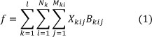
In equation (1), k represents the plot types. k = 1 indicates the single-crop plots, k = 2 indicates the double-crop plots, and so on. For each plot type k, i is indicative of the number of groups of crops that are grown in sequence throughout the year. For k = 1, Nk (or N₁) will be equivalent to 1. This will represent the group of crops that are grown all year around. For k = 2, Nk = 2. This will represent two groups of crops that are grown in sequence throughout the year. These are the summer and winter crop groups. The explanation is similar for k = 3, and so on. For each sequential crop group i, grown on plot k, j will represent the individual crops grown. For k = 1 and i = 1, j will be indicative of all the tree-bearing and perennial crops grown. For k = 2 and i = 1, j will be indicative of all the summer crops grown. For k = 2 and i = 2, j will be indicative of all the winter crops grown, and so on.

Equation (1) is subjected to the land and irrigated water allocation constraints given in Sections 2.6 and 2.7 below. The gross benefits B_kij that can be earned per crop must also satisfy the non-negative constraint given in Section 2.8 below.

2.6 Land constraints

Feasible solutions must satisfy the lower and upper bound constraints of the plot types k. This constraint is given in equation (2) below.

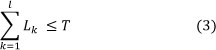
The sum of the hectares allocated for each plot type k must be less than or equal to T. This constraint is given by equation (3) below.

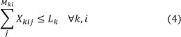
The sum of the hectares allocated for each crop j at stage i, on plot k, must be less than or equal to the total area of land allocated for agricultural production on plot type k. This constraint is given by equation (4) below.

The lower and upper bound constraints for each crop must be satisfied. This constraint is given by equation (5) below.

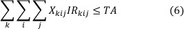
2.7 Irrigation constraints

The total volume of irrigated water that is required for the production of all crops within the year must be less than or equal to the total volume of irrigated water that can be supplied to the given area of land. This constraint considers that some crops may require more irrigated water than what is supplied per ha. It is therefore the responsibility of the farmer to distribute his supply of irrigated water efficiently. This constraint is given by equation (6) below.

2.8 Non-negative constraints

The gross profits that can be earned per crop must be greater than zero. This constraint is given by equation (7) below.

3 CASE STUDY

The Taung Irrigation Scheme (TIS) is situated in the Taung District, in the North West Province of South Africa. It adjoins the Vaalharts Irrigation Scheme (VIS) - one of the largest irrigation schemes in the world, with a total of 3,764 ha of irrigated land currently [2]. The irrigated water currently supplied to the TIS is drawn from the Vaal River, and is supplied via the Vaalharts Canal System, which also supplies irrigated water to the VIS. The irrigated water is supplied to the TIS at a basic quota of 8,417 m^-3 ha^-1annum^-1 to the farmers [2]. Located in the area of the TIS is the Taung Dam which, at full capacity, has a total volume of 62.97 million m^-3 of water. The dam was originally constructed to supply irrigated water to the TIS, but no infrastructure had been built to do so.

A recent survey [2] had been done to determine whether extending the existing TIS would be feasible in developing new irrigated areas. If it is found that the adjacent portions of land are viable, then the irrigated water supplied to the TIS will be drawn from the Taung Dam. The survey found that 3,315 ha are acceptable for agricultural production. It is also believed that agricultural production on this portion of land will match the high agricultural output of the neighbouring VIS. The current expansion of the TIS will cater for 175 people who had been previously excluded from the land. A total of 1,750 ha (10 ha per person) will now be allocated to them as restitution. As chosen by the local Department of Agriculture and the local farmers, the most suitable crops to be cultivated on this portion of land are those listed in Table 1 [2]. The crops consist of lucerne, which is grown all year around (y), and the rest of the crops, which are the summer (s) and winter (w) crops. Lucerne will be grown on single-crop plots of land, while the summer and the winter crops will be grown on double-crop plots of land.

 

 

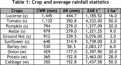
To determine solutions for the seasonal hectare allocations among the various competing crops that need to be grown, the crop water requirements (CWR) and the average rainfall (AR) statistics need to be determined. The AR values are the average amount of rain that is expected to fall during the growing months of each crop. The CWR is provided by the Department of Water Affairs and Forestry [2]. The average rainfall statistics are obtained from [10]. The producer price per ton (zAr¹ t^-1) of yield is determined from data from the Department of Agriculture, Forestry and Fisheries [11, 12]. The yield expected (t ha^-1) per crop is determined from data from the Kwa-Zulu Natal Department of Agriculture and Environmental Affairs[13]. The water quota of 8,417 m^-3ha^-1annum^-1 will remain the same. The cost of irrigated water is 8.77 cents/m^-3 [14].

 

4 METHODOLOGY

Swance (SI) irm Intelliges research inspired by observing the naturally intelligent behaviour of swarms of biological agents within their environment. Without any central control structure directing their movements, they seem to interact intelligently with each together, independently achieving their objectives [15]. These observations have led to the development of many effective SI optimisation algorithms. The algorithms typically represent the individual behaviour of the biological agents, which are represented by a set of simple rules.

SI algorithms have provided effective solutions to many real-world optimisation problems that are NP-Hard in nature. This research investigates the effectiveness of employing three relatively new SI metaheuristic algorithms in solving the ACP problem at the TIS. The algorithms investigated are Cuckoo Search (CS), Firefly Algorithm (FA), and Glow-worm Swarm Optimisation (GSO). To determine the relative merits of the solutions provided by these algorithms, their solutions will be compared against the solutions of a traditional population-based metaheuristic algorithm, the Genetic Algorithm (GA). Brief descriptions of these algorithms are given in the subsections below.

4.1 Cuckoo Search

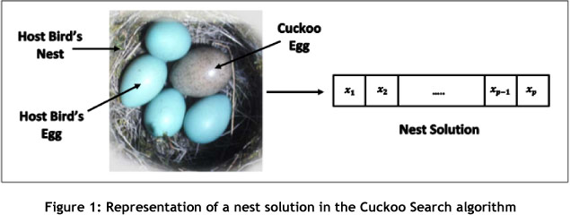
CS [16] is inspired by the parasitism of some cuckoo bird species. These birds aggressively reproduce and then abandon their eggs in the nests of other bird species as hosts. Some host birds behave aggressively and eject the alien eggs upon discovering an intrusion. Others simply leave their nests and build new nests elsewhere. Each egg in the host bird's nest represents a possible solution. The goal of the CS algorithm is to replace an inferior solution in the host bird's nest with a potentially better solution. This is represented by a newly-laid egg. There are three guiding rules governing the CS algorithm:

1. Each bird lays one egg at a time. The egg gets placed randomly among the host bird nests.

2. The nest with the highest fitness value will get carried over to the next generation.

3. The number of host bird nests is fixed. The probability of a host bird discovering an intrusion is set at a constant value of ρ_a є [0,1].

In generating a new solution, the random-walk is best performed by using Levy flights. The Levy flight of cuckoo i is performed using equation (8).

where δ is drawn from a standard normal distribution with mean 0 and standard deviation of 1. δ determines the direction of movement. s is the step size. This determines the distance of the random walk. Determining s is tricky. If s is too big, then x_i (t + 1) will be too far away from x_i(t). If s is too small, then x_i (t + 1) will be too close to x_i(t) to be significant. One of the most efficient algorithms used to calculate s is Mantegna's algorithm [16]. Using Mantegna's algorithm, s can be calculated by using equation (9).

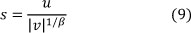
where u and v are drawn from a normal distribution, and 0 < β < 2.

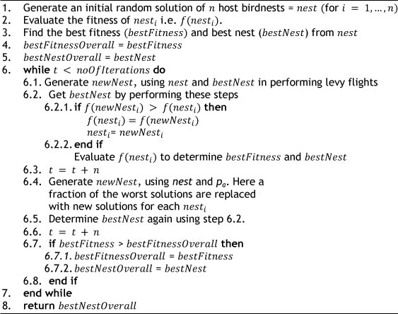
CS is implemented in this research by first randomly generating a population of n host bird nest solutions, i.e. nest (for i = 1, ..., n). Each egg in nest_i is represented by a randomly-generated number that falls between 0 and 1. The fitness value of each nest i is then calculated. The best fitness value found in the population and its corresponding solution is then recorded in variables bestFitness and bestNest respectively.

At each iteration of the algorithm, a new population of nests (newNest) is generated using nest and bestNest. Each newNest_i is determined in moving nest_i in the direction of bestNest using equation (8). The best nest solution from newNest is then determined and compared against bestNest to check if an improved solution has been found. If the solution improves on bestNest, then bestNest is replaced with this improved solution. Intrusion is implemented thereafter on each egg in newNest_i if ρ_a < rand, where rand is a randomly generated number between 0 and 1. If ρ_a < rand then a new value for the egg is generated at random. At this point, the best solution from newNest is determined and is again compared against bestNest to see if an improved solution is found.

bestNest will contain the best solution found by the algorithm, and this will be returned when the stopping criterion is met.

The algorithm for CS is as follows:

 

 

A visual representation of a nest solution in CS is given in Figure 1 below, which shows the eggs of a host bird and that of a cuckoo bird in the nest of a host bird. Each egg x_l (V l = 1, ..., ρ) represents a possible solution in the solution of a nest.

4.2 Firefly

FA [16] is inspired by the ability of fireflies to emit light (bioluminescence) in order to attract other fireflies for mating purposes. There are three guiding rules governing this algorithm:

1. Fireflies are attracted towards brighter fireflies, regardless of their sex.

2. The attractiveness of a firefly is related to its brightness. However, it is assumed that the brightness decreases with distance. The brightest firefly moves randomly.

3. The brightness of the firefly is a function of the problems objective.

Attractiveness: The attractiveness of a firefly is given by equation (10).

Here, r is the distance between any two fireflies. β₀ represents the initial attractiveness at r = 0. y is an absorption coefficient. It controls the decrease in the intensity of light.

Movement: The movement of a less attractive firefly i towards a more attractive firefly j is given by equation (11).

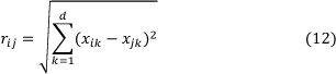
where x_i is the current position of the firefly within the solution space. The combination of the elements in the second term represents the firefly's attractiveness, as seen by the other fireflies. The third term represents a random adjustment in the movement of the firefly. α is a scaling parameter, αϵ [0,1]. rand is a uniformly distributed random number, rand ϵ (0,1). r_ij represents the distance between fireflies i and j. It is calculated using the Cartesian distance [16] given in equation (12).

FA is implemented in this research by first randomly generating a population of fireflies, i.e. fireflyLocations (for i = 1 ... n). Each element of each firefly, i.e. fireflyLocations_il 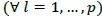, is represented by a randomly generated number that falls between 0 and 1. The light intensity, or fitness value, of each firefly is then calculated and stored in the variable fireflyFitness_i.

At each iteration, the fireflies in the population are sorted in descending order according to their fitness values. The fitness value of every firefly is then compared to the fitness value of every other firefly j (for j = 1 ... n). If fireflyFitness_i < fireflyFitness_j then firefly i moves in the direction of firefly using equation (11).

When the stopping criterion is met, the solution returned will be the first solution in fireflyLocations after the sorted order is maintained, i.e. fireflyLocations₀.

The FA algorithm is as follows:

Initialize α, β₀, γ and noOfIterations

 

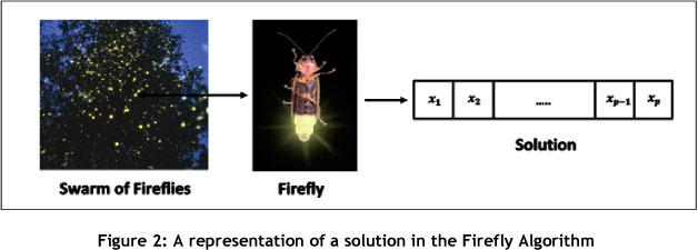
A visual representation of a solution in FA is given in Figure 2 below, which shows a swarm of fireflies. The position of each firefly represents a solution within the solution space. Its position is determined by the variables . The position of each firefly will determine the bioluminescence emitted.

4.3 Glow-worm Swarm Optimisation

The Glow-worm Swarm Optimisation (GSO) [17, 18] is inspired by the natural behaviour of glow-worms in emitting a luminescent property called luciferin, in order to attract other glow-worms. Glow-worms with larger emissions of luciferin are considered more attractive. A glow-worm moves towards a brighter glow-worm if it lies within its range of view.

Initially, glow-worms are distributed randomly throughout the solution space. At any point in time t, the state of a glow-worm i is represented by its luciferin level I_i (t), its position x_i(t), and its vision range r_i(t). During each iteration, these variables are updated, and it describes the movement of the glow-worms within the solution space. The luciferin update is given by equation (13).

where is the luciferin decay constant (0 < ρ < 1). is the luciferin enhancement constant. is the evaluation of the objective function, at time t.

To update the position of each glow-worm i, a set of neighbours N_i (t) needs to be determined. A glow-worm j is considered a neighbour of glow-worm i, if j falls within i's vision range r_t(t), and if I_i (t) < l_j(t). A glow-worm j is then selected from N_i (t), using roulette wheel selection. Glow-worm i then moves in the direction of glow-worm j using equation (14).

where st is a constant step size.

Lastly, the vision range r_i(t) needs to be updated, using equation (15).

Here, r_s, β and Nd are constant values. rs is the maximum vision range, β is the rate of change of the neighbourhood range, and Nd is the maximum number of neighbours that glow-worm i is allowed to have.

GSO is implemented in this paper by first randomly generating a population of n glowworms, i.e. glowworm (for i = 1, ..., n). Each element of each glow-worm, i.e. glowworm_il , is represented by a random number which falls between 0 and 1. The fitness values of each glowworm_i are then calculated. The best fitness value and its corresponding solution is then stored in variables bestFitness and bestLocation, respectively.

At each iteration, the movement of each glow-worm i is performed using equations (13), (14) and (15). The best glow-worm from the newly-generated population is then determined, and its fitness value is cross-referenced against bestFitness. If its fitness value improves upon bestFitness, then bestFitness and bestLocation are replaced with the fitness value and the solution of the best glow-worm found. When the stopping criterion is met, bestLocation is returned.

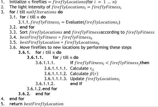
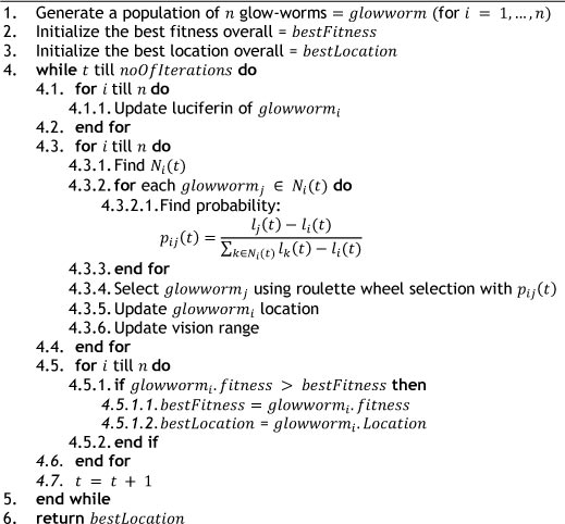
The GSO algorithm is as follows:

A visual representation of a solution in GSO is given in Figure 3 below, which shows a swarm of glow-worms. The position of each glow-worm within the solution space represents a solution. Its position is determined by the variables . The position of each glow-worm will determine the luciferin emitted.

4.4 Genetic Algorithm

The Genetic Algorithm (GA) [19] is inspired by the process of natural evolution. By modelling evolutionary processes such as selection, crossover, and mutation, a population of chromosomes (genotypes of the phenotypes or individuals) evolves from one generation to the next. Chromosomes are binary encoded for discrete optimisation problems or real-value encoded for continuous optimisation problems [20].

GA starts off with an initial, randomly-generated population of chromosomes/solutions. Each solution has an associated fitness value that indicates the individuals' strength. Using these fitness values, or not, pairs of solutions are stochastically selected from the current population at each generation. Using techniques such as crossover and mutation, these pairs of solutions will produce offspring solutions. The offspring solutions form the new population, which represent the next generation. This process will continue for a specified number of generations or until a satisfactory fitness value has been found.

Selection is done using techniques such as the roulette wheel selection and random selection [20]. Roulette wheel selection considers the fitness value of the solutions, while random selection does not. When a pair of solutions is selected, the crossover process generates offspring solutions that are a recombination of their parent solutions. Recombination is done using techniques such as n-point crossover, uniform crossover, and arithmetic crossover [20]. The 'genes' of the offspring have a probability of undergoing mutation. Mutation reduces the risk of premature convergence. Premature convergence occurs when the heuristic algorithm becomes trapped within a local neighbourhood structure of the solution space, in which the local optimal solution is not 'close' enough to the global optimal solution.

The implementation of GA in this research was done using real-value encoding and uniform crossover. Initially a population of n chromosomes/solutions is generated, i.e. population (for i = 1, ... ,n). Each gene in each chromosome, i.e. population_il , is represented by a random number between 0 and 1. The fitness value of each solution in the population is then calculated, and the best solution, according to the best fitness value found, is recorded in the variable bestIndividual.

At each iteration of the algorithm, and until the new population is created, two parent solutions are selected from the previous population using roulette wheel selection. Given a predetermined crossover rate (cRate), crossover is performed at each index of the adjacent genes of the parent solutions if rand < cRate. rand is a randomly generated number between 0 and 1. If rand < cRate then the adjacent genes will be swapped in generating the offspring solutions, or else the genes will remain the same in being passed over to the offspring.

Once the offspring solutions have been generated, then mutation is performed on each gene of the offspring solutions in using a predetermined mutation rate (mRate). If rand < mRate then mutation is performed on each gene by simply assigning a new randomly generated number, rand. Once mutation is complete, the offspring are added to the new population.

When the new population is generated, the best solution from the population is determined and is compared against bestIndividual. This is to check whether an improved solution has been found. If it has, then bestIndividual is replaced by the improved solution. When the stopping criterion is satisfied, bestIndividual is returned. This is the best solution found by the algorithm.

The algorithm for GA used in this research is as follows:

 

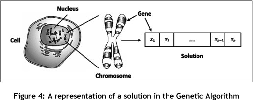
A visual representation of a solution found in GA is given in Figure 4 below, which shows a population of chromosomes within the nucleus of a cell. Each chromosome consists of genes, , which make up a solution.

 

 

5 TESTING AND EVALUATION

The non-heuristic specific parameters required for the execution of the algorithms had been set according to the values given in Tables 2 and 3. The lower and upper bound settings for the different plot types are given in Table 2.

 

 

 

 

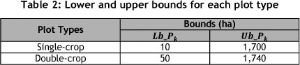
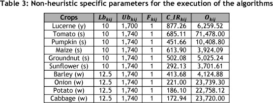
Table 3 gives the lower and upper bound settings, the land coverage fraction values, the cost of irrigated water, and the operational costs for each crop. The large differences between the lower and upper bound values were to investigate the ability of the heuristic algorithms to determine solutions in a larger solution space. F_kij ϵ [0,1]. C_IR_kij is the cost of the irrigated water per hectare per crop (ZAR ha^-1). Operational cost 0_kij is set to a third of the producer price per ton of yield (ZAR ha^-1).

The initial parameters for the heuristic algorithms were set as follows:

•  CS - The number of host bird nests n was set at 20. The noOfIterations was set at 100,000. ρ_α was set at 0.25.
•  FA - The number of fireflies n was set at 20. The noOfIterations was set at 5,000. α was set at 0.25, β₀ at 0.2 and γ at 1.
•  GSO - The number of glow-worms n was set at 20. The noOfIterations was set at 5,000. I₀ was set at 1, r₀ at 1.2, rs at 1.5, ρ at 0.4, γ at 0.6, β at 0.08, st at 0.3 and Nd at 10.
•  GA - The number of individuals n was set at 20. The maxNoOfGenerations was set at 5,000. cRate was set at 0.8. mRate was set at 0.05 (1/n).

ρ_α was set according to the setting given in Xin-She Yang's Matlab^® implementation of CS [21]. α, β₀ and γ were set according to the settings given in Xin-She Yang's Matlab^® implementation of an m-dimensional Firefly Algorithm [22]. For GSO, ρ, γ, β, and st were set according to the settings given in [23]. l₀, r₀ and rs are problem specific parameters. Nd was set to half of the number of glow-worms n. For GA, cRate was set at 0.8. This value was used after several tests had been performed to determine the best probable crossover rate to use.

In order to compare the heuristic algorithms fairly, each algorithm was set to the same 'population' size, i.e. n = 20. The noOfIterations (for CS, FA, and GSO) and the maxNoOfGenerations (for GA) ensured that each algorithm executed for 100,000 objective function evaluations. Each algorithm was run 100 times, using randomly-generated population sets for each run.

In order to ensure fairness, the 100 different population sets had been initially randomly generated. For explanation, we mathematically denote each population set as popi, for i = 1, ... ,100. Then, for each run i, popi was used as the input population set for each of the heuristic algorithms. This means that for run i = 1; CS, FA, GSO and GA were run using pop₁, for run i = 2; CS, FA, GSO and GA were run using pop₂, and so on until i = 100. From the 100 best solutions determined by each heuristic algorithm, the results of the best and average solutions have been documented. Using the populations of the 100 best solutions determined by each heuristic algorithm, the 95% Confidence Interval² values have been calculated for the execution times and for the fitness values (total gross profits). The results are explained below.

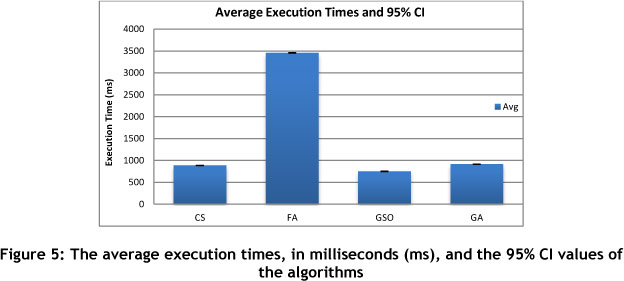
Table 4 gives the statistics of the average execution times (AVG) in milliseconds (ms), and the 95% Confidence Interval (95% CI) values of each heuristic algorithm.

 

 

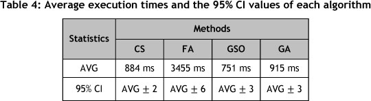
From Table 4 we observe that FA took the longest time to execute. The average execution times of CS, GSO, and GA were all comparable. The relatively large average execution time of FA is due to its nested 'for' loop. In this 'for' loop, each firefly's fitness value is compared with the fitness value of every other firefly. This was shown to be computationally expensive.

The execution time of GSO is the fastest. This is due to the limitation on the maximum number of neighbours that a glow-worm is allowed to have. As the number of iterations increases, the vision ranges of the glow-worms will decrease. This will cause the glowworms to become more separated in searching the local neighbourhood structures of the solution space. This separation will reduce the number of glow-worms considered in searching for neighbours, which will speed up the execution process.

The 95% CI values from Table 4 mean that we can be 95% certain that the 100 execution times of each algorithm have fallen within those interval estimates. By observing those CI values we conclude that the execution times of the algorithms have been fairly consistent. A visual representation of the statistical values from Table 4 is given in Figure 5 above, where the 95% CI values are represented by the black interval estimates.

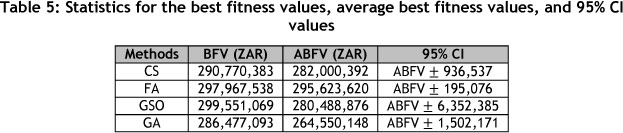
Table 5 gives the statistical values of the overall best (BFV) and average best (ABFV) fitness values for each heuristic algorithm. The fitness values are the total gross profits earned. The 95% CI values for the fitness value populations of each algorithm are also given.

From Table 5 it is observed that GSO determined the highest BFV. This is followed by FA, CS, and then GA. On average FA performed the best. This is followed by CS, GSO, and then GA. Each SI algorithm determined superior solutions compared with GA.

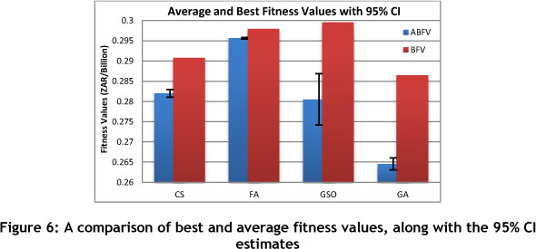
A graphical comparison of the algorithms' best and average fitness values, as determined from Table 5, is given in Figure 6. The 95% CI values are represented by the black interval estimates, over the average fitness values.

The solutions found by the algorithms were in a solution space of constantly changing plot type hectare allocations. The hectare allocations for each plot type had to be determined first, before the hectare allocations of the crops, and had to satisfy the land constraints given in Section 2.6.

For each algorithm, the best solution determined from the 'population' of solutions at iteration t, for plot type hectare allocations p, will not necessarily be the best solution at iteration (t + 1) for plot type hectare allocations (p + 1). The change in the plot type hectare allocations at iteration (t + 1) will change the crop hectare allocations accordingly, so that the land constraints do not break. The constantly changing dimensions of the solution space make it very difficult for the algorithms to perform exploitation³. This makes it difficult to determine effective solutions.

Under the circumstance of the constantly changing dimensions of the solution space, FA performed most consistently. This is confirmed by its low 95% CI fitness value. Having the highest average best fitness value also means that FA has been the strongest heuristic algorithm for this particular ACP problem. CS had the second-lowest 95% CI fitness value. This is followed by GA, and then GSO.

Although GSO's average performance is worse than CS, its best fitness value and its high 95% CI fitness value prove that it determined many good solutions. However, it also determined many poor solutions, which is the reason for its lower average.

The strength of FA and GSO in determining the best fitness solutions overall is attributed to the algorithms' versatility in being able to accept both improved and worse solutions at each iteration.

In FA, as the fireflies are attracted towards brighter fireflies, some will accept improved solutions, while others will accept worse solutions within the local neighbourhood structures of the solution space. The solutions that are classified as being either improved or worse depend entirely on the plot type hectare allocations at iteration . However, at iteration (t + 1), the sorting of the fireflies will take place according to the plot type hectare allocations (p + 1) and not p. Therefore, what appeared to be improved solutions at iteration for might not necessarily be improved solutions at iteration (t + 1) for (p + 1). Similarly, what appeared to be worse solutions at iteration t for p might not necessarily be worse solutions at iteration (t + 1) for (p + 1). The versatility of FA in accepting both improved and worse solutions has been shown to be very valuable for this particular optimisation problem.

In GSO, a glow-worm will accept an improved or worse solution in moving towards another glow-worm with a higher level of luciferin than itself. Similarly to FA, this ability has been shown to be very valuable for this particular optimisation problem. GSO's average best fitness value is, however, relatively low compared with FA and CS. Interestingly enough, it also has the highest 95% CI fitness value. The reason for the instability in its performances is due to its ability deliberately to cause group-like separations of the glow-worms throughout the neighbourhood structures of the solution space. The separations are achieved by reducing the glow-worms' vision ranges as the number of iterations increase, and in limiting the maximum number of neighbours that a glow-worm is allowed to have. The group-like separations result in fewer glow-worms searching the local neighbourhood structures of the solution space. This technique's strength is in exploration⁴, but it is lacking in terms of exploitation. Strong exploration abilities are beneficial for this optimisation problem due to the constantly changing plot type hectare allocations. However, the 'weakness' in its exploitation ability reduces the probability of its performing consistently on average. This explains its relatively low average best fitness value.

For each host bird's nest solution in the 'population', CS only accepts new nest solutions if they improve upon the host bird nest solutions in the population. The new nest solutions are generated by using the best nest solution from the previous iteration in performing Levy flights. However, as explained earlier, what appeared to be the best nest solution at iteration (t -1) for plot type hectare allocations (p - 1) will not necessarily be the best nest solution at iteration t, using plot type hectare allocations . Therefore, due to the constant changes in the dimensions of the solution space, performing Levy flights will not result in the most effective exploitation. The probability of the host bird's discovery of intrusions facilitates exploration. This gives CS its best chance of determining improved solutions.

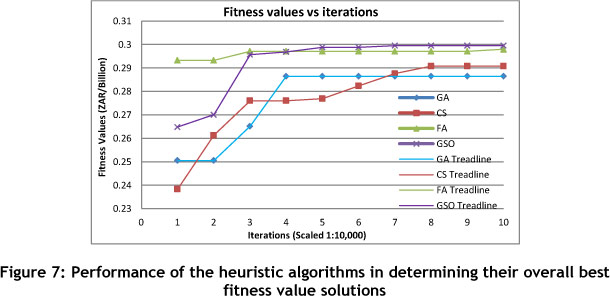
Figure 7 shows the run-time performances of the heuristic algorithms during the determination of their best fitness value solutions. FA found improved solutions at the fastest rate up until around 25,000 objective function evaluations. At this point GSO determined a solution similar to FA. At around 63,000 objective function evaluations, GSO had determined the best fitness value of all the heuristic algorithms. FA found its best fitness value at around 90,000 objective function evaluations. Its improvement was not enough to be the best overall. CS showed steady increases in determining improved solutions. At around 70,000 objective function evaluations, CS found a neighbourhood within the solution space that had a solution that was better than GA's best solution. GA found its best solution at around 34,000 objective function evaluations.

Table 6 gives the statistics of the irrigated water requirements (IWR) and the variable costs of production (VCP) for the best solution determined by each of the heuristic algorithms. FA required the least amount of irrigated water. At a cost of ZAR 0.0877 m^-3, the cost of this irrigated water is ZAR 1,487,581. CS's IWR value was only 9,374 m^-3 more than FA. GSO's IWR value was 90,761 m^-3 more than FA. At a water quota of 8,417 m^-3ha^-1annum^-1, FA's IWR value would have supplied irrigated water to 10 ha less than GSO's value. GA's irrigated water requirement is the highest. The relative increases in the variable costs of production (VCP) for each SI algorithm, compared with GA, are acceptable considering the increased total gross profits earned.

 

 

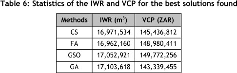
A graphical representation of the IWRs, as determined from Table 6, is shown in Figure 8.

 

 

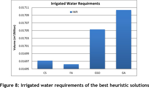
Table 7 gives the plot type hectare allocations for the best solution found by each algorithm. Each heuristic algorithm determined that the total gross profits could be increased by allocating more land for the double-crop plots. This was as a result of Lucerne's high irrigated water requirement and low producer price t^-1.

 

 

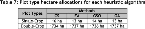
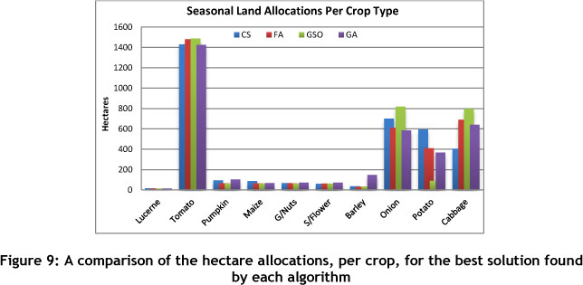
Figure 9 gives a graphical comparison of the seasonal hectare allocations of each crop, for the best solution determined by each heuristic algorithm.

For the single-crop plots of land, each algorithm determined similar hectare allocations for lucerne. For the double-crop plots of land, each algorithm allocated the most land to tomato, onion, and cabbage. The large hectare allocations for tomato are due to its high yield ha^-1 and high producer price t^-1. Similar hectare allocations were determined for pumpkin, maize, ground nuts, and sunflower. GA's relatively higher hectare allocation for barley contributed to its relatively poor best performance.

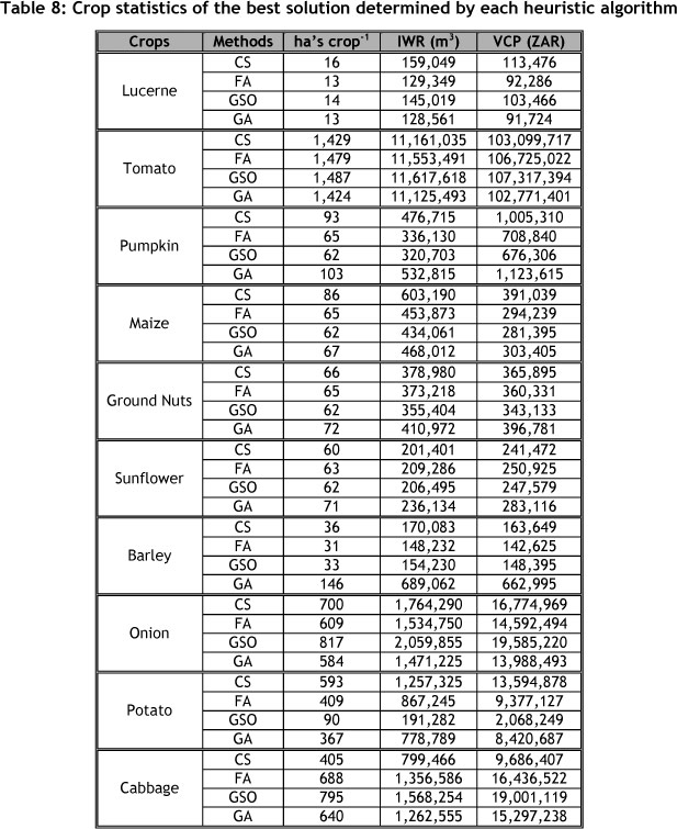
Table 8 gives the statistical values of each crop's hectare allocations (ha's crop^-1), irrigated water requirements (IWR), and variable costs of production (VCP) for the best solution determined by each heuristic algorithm.

The program was written in the Java programming language, using the Netbeans^® 7.0 Integrated Development Environment. All simulations were run on the same platform. The computer used had a Windows^® 7 Enterprise operating system, an Intel^® Celeron^® Processor 430, 3 GB of RAM, and a 500GB hard-drive.

 

6 CONCLUSION

Shortages in food supply and increases in population growth have increased the need for food production. To try to meet this growing demand for food, it is important that new irrigation schemes be developed to increase agricultural output.

Planning new irrigation schemes requires that optimised solutions be found for the seasonal hectare allocations of the crops that need to be grown within the year. The solutions found must maximise the total gross profits that can be earned, to make the most efficient use of the limited resources available for agricultural production. Determining solutions to this problem is referred to as annual crop planning (ACP), an NP-Hard optimisation problem in agricultural planning.

This research has introduced a new ACP mathematical model, which is intended to be used to determine solutions to the ACP problem at a new irrigation scheme. The case study in this paper is the Taung Irrigation Scheme (TIS), situated in the North West Province of South Africa. The irrigation scheme is currently being expanded to cater for an extra 1,750 hectares of irrigated land. This portion of land is required to grow 10 different types of crops. In order to determine solutions for this ACP problem, three relatively new Swarm Intelligence (SI) metaheuristic algorithms have been investigated. These algorithms include Cuckoo Search (CS), Firefly Algorithm (FA), and Glow-worm Swarm Optimisation (GSO). To determine the relative merits of their solutions, they have been compared against the solutions of another popular population-based metaheuristic algorithm, the Genetic Algorithm (GA). To ensure fairness in the performances of the heuristic algorithms, their algorithm-specific parameters had used recommended settings. Other parameter settings, such as the 'population' sizes, the initial population sets, and the number of objective function evaluations per run, were all set to be the same. Each heuristic algorithm was run 100 times. From these 100 runs, the overall best and average solutions of each heuristic algorithm were documented.

The results show that GSO determined the overall best solution. This was followed by FA, CS, and then GA. On average, FA performed the best, followed by CS, GSO, and then GA. FA showed the lowest 95% Confidence Interval (95% CI) fitness value. This proved that, in a solution space of constantly changing dimensions, FA performed most consistently. In this research, FA was the strongest heuristic algorithm. The disadvantage of FA was its relatively higher average execution time. Although GSO's average performance was worse than CS, its best solution and its high 95% CI fitness value proved that it had determined some very good solutions. GSO also had the fastest average execution time. Of all the heuristic algorithms, GA performed the worst overall. An advantage of FA and CS is their relative ease of implementation in developing object-oriented versions of the algorithms, compared with GSO. CS requires the fewest parameter settings.

Possible future work will be to extend this ACP mathematical model (or formulate new models) to take into account factors such as the dynamic pricing of crops and caloric requirements. An investigation into the effectiveness of employing local search metaheuristic techniques in determining solutions to this ACP problem might also be considered.

 

REFERENCES

[1] Schmitz, G.H., Schütze, N. & Wöhling, T. 2007. Irrigation control: Towards a new solution of an old problem. IHP/HWRP-Berichte, Vol. 5. International Hydrological Programme (IHP) of UNESCO and the Hydrology and Water Resources Programme (HWRP) of WMO, Koblenz, Germany.         [ Links ]

[2] Department of Water Affairs and Forestry, 2008. Vaal River system: Feasibility study for utilization of Taung Dam water: Irrigation planning and design. Report Number P WMA 10/C31/00/0908. [Online] Available: http://www.dwaf.gov.za/.         [ Links ]

[3] Pant, M., Radha, T., Rani, D., Abraham, A. & Srivastava, D.K. 2008. Estimation using differential evolution for optimal crop plan. Lecture Notes in Computer Science, 5271, pp. 289-297.         [ Links ]

[4] Pant, M., Thangaraj, R., Rani, D., Abraham, A. & Srivastava, D.K. 2009. Estimation of optimal crop plan using nature inspired metaheuristics. World Journal of Modelling and Simulation, 6 (2), pp. 97-109.         [ Links ]

[5] Georgiou, P.E. & Papamichail, D.M. 2008. Optimization model of an irrigation reservoir for water allocation and crop planning under various weather conditions. Irrigation Science, 26(6), pp. 487-504.         [ Links ]

[6] Wardlaw, K. & Bhaktikul, K. 2007. Application of genetic algorithms for irrigation water scheduling, Irrigation and Drainage, 53, pp. 397-414.         [ Links ]

[7] Sarker, R. & Ray, T. 2009. An improved evolutionary algorithm for solving multi-objective crop planning models. Computers and Electronics in Agriculture, 68(2), pp. 191-199.         [ Links ]

[8] Raju, K.S. & Kumar, N.D. 2004. Irrigation planning using genetic algorithms. Water Resources Management, 18(2), pp. 163-176.         [ Links ]

[9] Reddy, J.M. & Kumar, N.D. 2007. Optimal reservoir operation for irrigation of multiple crops using elitist-mutated particle swarm optimization, Hydrological Sciences, 52(4), pp. 686-701.         [ Links ]

[10] Maisela, R.J. 2007. Realizing agricultural potential in land reform: The case of Vaalharts Irrigation Scheme in the Northern Cape Province. Master of Philosophy thesis, University of Western Cape, Cape Town, South Africa.         [ Links ]

[11] Department of Agriculture, Forestry and Fisheries, 2012. Trends in the agricultural sector 2012. [Online]. Available: http://www.daff.gov.za/docs/statsinfo/Trends2011.pdf.         [ Links ]

[12] Department of Agriculture, Forestry and Fisheries 2012. Abstract of agricultural statistics 2012. [Online]. Available: http://www.nda.agric.za/docs/statsinfo/Ab2012.pdf.         [ Links ]

[13] Department of Agriculture & Environmental Affairs, 2012. Expected yields. [Online]. Available: http://www.kzndae.gov.za/.         [ Links ]

[14] Grove, B. 2008. Stochastic efficiency optimisation analysis of alternative agricultural water use strategies in Vaalharts over the long- and short-run. Ph.D. thesis. Department of Agricultural Economics, University of the Free State, Bloemfontein, South Africa.         [ Links ]

[15] Blum, C. & Merkle, D. 2008. Swarm intelligence introduction and applications. Springer-Verlag Berlin Heidelberg.         [ Links ]

[16] Yang, X.S. 2010. Nature-inspired metaheuristic algorithms, 2^nd edition, Luniver Press, United Kingdom.         [ Links ]

[17] Krishnand, K.N. & Ghose, D. 2009. Glowworm swarm optimisation for simultaneous capture of multiple local optima of multimodal functions. Swarm Intelligence, 3, pp. 87-124.         [ Links ]

[18] Krishnand, K.N. & Ghose D. 2009. Glowworm swarm optimisation: A new method for optimizing multimodal functions. International Journal of Computational Intelligence Studies, 1(1), pp. 93-119.         [ Links ]

[19] Holland, J.H. 1975. Adaptation in natural and artificial systems. University of Michigan Press, Ann Arbor, MI.         [ Links ]

[20] Eiben, A.E. & Smith, J.E. 2003. Introduction to evolutionary computing, 1^st edition, Springer, Natural Computing Series.         [ Links ]

[21] Yang, X. 2013 Cuckoo Search Algorithm. [Online] Available: http://www.mathworks.com/matlabcentral/fileexchange/29809-cuckoo-search-cs-algorithm/content/cuckoo_search.m.         [ Links ]

[22] Yang, X. 2013. Firefly Algorithm. [Online] Available: http://www.mathworks.com/matlabcentral/fileexchange/29693-firefly-algorithm/content/fa_ndim.m.         [ Links ]

[23] Zhao, G., Zhou, Y. & Wang, Y. 2012. The glowworm swarm optimization algorithm with local search operator. Journal of Information & Computational Science 9(5), pp. 1299-1308.         [ Links ]

 

 

1 ZAR stands for Zuid-Afrikaanse Rand. It is the Dutch translation of "South African Rand", the South African currency.
2 In statistics a Confidence Interval (CI) indicates the reliability of an interval estimate of population parameters. 95% CI means to be 95% certain that the population parameters will lie within the interval estimate range.
3 Exploitation is the act of searching or travelling within a local neighborhood structure of the solution space in the hope of determining the local optimum solution. It is a local search technique.
4 Exploration is the act of searching or travelling within the solution space in the hope of determining the neighborhood structure that contains the global optimum solution. It is a global search technique.