GENERAL ARTICLES

 

Application of the aviation derived maintenance free operating period concept in the South African mining industry

 

 

Amir Al Shaalane^I; P.J. Vlok^II

^IDepartment of Industrial Engineering. University of Stellenbosch. Stellenbosch, South Africa. amiralshaalane@gmail.com
^IIDepartment of Industrial Engineering. University of Stellenbosch. Stellenbosch, South Africa.pjvlok@sun.ac.za

 

 

---

ABSTRACT

This paper analyses the use and possible application of the concept of the maintenance free operating period (MFOP), derived from the aviation sector, in the mining industry. The traditionally used reliability requirement, mean time between failure (MTBF), has been found to have several inherent problems with its application and definition. These problems are explained in this paper. It also provides a brief overview of the field of physical asset management (PAM), the overall domain of the research, and thereafter provides a characterisation of MTBF and its current use in the mining industry. MFOP is then introduced and contrasted with MTBF. A methodology for the analysis of MFOP performance is introduced and then applied to a case study conducted at an Anglo American platinum mine.

---

OPSOMMING

Hierdie verslag ontleed die nut en moontlike toepassing van die konsep 'instandhoudingsvrye bedryfstydperk' (MFOP), wat oorspronklik uit die lugvaartsektor kom, in die mynbedryf. Die tradisionele betroubaarheidsvereiste 'gemiddelde tydsduur tussen weierings' (MTBF) blyk etlike inherente probleme te hê wat toepassing en omskrywing betref, wat óók hierin bespreek word. Die navorsing bied voorts 'n bondige oorsig van die terrein van fisiese batebestuur (PAM), synde die oorkoepelende gebied waarop dié studie tuishoort, en beskryf daarná die MTBF-vereiste en die huidige aanwending daarvan in die mynbedryf. MFOP word dan bekend gestel en met MTBF vergelyk. 'n Metode vir die ontleding van MFOP-werkverrigting word voorgestel en uiteindelik op 'n gevallestudie by 'n myn van Anglo American platinum toegepas.

---

 

 

1 INTRODUCTION

In the current extremely competitive industrial environment, optimised maintenance decisions and programmes are becoming increasingly important to asset-centric organisations. Trillions of dollars are spent every year around the world to maintain plant systems and equipment. Heng et al. [1] state that, in 1981, plants in the United States had already spent more than US $600 billion to maintain their critical plant systems. It is a massive industry, not only in terms of expenditure, but also in terms of maintenance activities; it therefore needs optimised maintenance activities to gain maximum benefit for the operator at the lowest cost. This vital industry recently saw the creation and implementation of the British Standard Publicly Available Specification 55 (PAS 55), which deals specifically with PAM. This has been bolstered even further by the forthcoming creation of an International Organization for Standardization (ISO) standard on PAM from the Publicly Available Specification (PAS) 55 standard, to be known as ISO 55000. Within PAM and PAS 55 there are certain primary requirements to optimise asset management activities: acquire, utilise, maintain, and renew. This research concerns itself with the 'maintain' asset management activity within the PAS 55 realm.

As with most industries, in maintenance there is a constant drive to improve the status quo. Mobley [2] points out that maintenance is one of the driving factors behind reliable and efficient operations. However, many industries still knowingly perform ineffective maintenance action. As a result there is a constant push, especially in the engineering discipline, to optimise methods and practices.

An important part of maintenance is reliability and the reliable operation of equipment. To quantify reliability, reliability metrics or maintenance interval metrics are used. These are an intrinsic and fundamental part of maintenance, which in turn makes up a significant segment of the life cycle of activities performed on an asset. This research specifically concerns itself with the definition of reliability metrics and their application. These are discussed in the sections that follow.

 

2 PHYSICAL ASSET MANAGEMENT

To understand the relatively new term of PAM correctly, we start with a definition. The one below comes from Vanier [3],[4]:

... a systematic process of maintaining, upgrading and operating physical assets cost effectively. It combines engineering principles with sound business practices and economic theory, and it provides tools to facilitate a more organised, logical approach to decision-making. Thus, asset management provides a framework for handling both short- and long-term planning.

It is important to note that PAM should not be confused with the well-known term 'asset management', which stems from the financial sector. Hastings [5] calls this form of asset management the "accounts view", where assets are split into the two financial terms of fixed and current assets. Amadi-Echendu et al. [6] point out that there should be a clear distinction between 'engineering' asset objects and 'financial' assets. Financial assets are traded on the stock exchange or form part of patent rights, and only exist as contracts between legal entities. Engineering objects can be categorised as items such as inventories, equipment, and land and buildings; what differentiates these from financial objects is that they can exist independently from any organisation or contract. To avoid confusion, PAM is also sometimes referred to as 'engineering asset management'.

PAM concerns itself not only with maintenance, but also with the entire life cycle of physical assets, and the alignment of the organisation's assets with the overall goals of the organisation. Both Amadi-Echendu [7] and Woodhouse [8] make the point that aligning utilisation and management towards desired stakeholder performance is a key challenge for PAM. PAM represents [8] the best sustainable mix of both 'asset care' and 'asset exploitation'. Here, asset care is the high level term coined to describe the mix of tactical and non-tactical maintenance activities that are performed, and asset exploitation describes the use of an asset to meet some organisational objective or goal.

Due to PAM's intrinsic and cross-functional nature within an organisation, it has yielded the formation of a standard on the topic. The PAS 55 standard was created from the need to formalise PAM, and attempts to bridge the gap usually found between senior management and lower level maintenance management. PAS 55 is published by the British Standards Institution, and is split into two parts [9]: PAS 55-1 deals with the specifications for the optimised management of physical assets; and PAS 55-2 deals with the guidelines for the application of PAS 55-1. The widespread acknowledgment of the PAS 55 standard within industry is now being formalised into an ISO standard, and will eventually be known as ISO 55000.

PAS 55 [9] defines PAM in a manner similar to that of Vanier [3], with this definition:

the systematic and coordinated activities and practices through which an organisation optimally and sustainably manages its assets and asset systems, their associated performance, risks and expenditures over their life cycles for the purpose of achieving its organisational strategic plan.

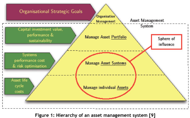
Similarities can be seen in both definitions. They both describe how PAM encompasses a much broader and different set of objectives and activities than the traditional term associated with PAM - maintenance. Figure 1 shows the hierarchy of an asset management system, and within that, where this research places itself.

This research deals with the management of assets or asset systems and, therefore, more specifically with maintenance on these assets; and with their performance assessment and improvement. PAS 55 [9] specifically emphasises communication between the organisation's strategic plan and the on-the-ground daily activities of individual departments.

 

3 CURRENT USE OF MEAN TIME BETWEEN FAILURE (MTBF) IN MINING

The mining industry can very clearly be characterised as an asset centric or asset intensive industry. Large numbers of physical assets need to interact closely to achieve the organisation's strategic goals, and thus create a profit for the organisation. As previously stated, PAS 55 [9] draws attention to the fact that there needs to be overall organisational alignment at all levels to achieve the overall organisational PAM strategy.

Mining processing operations require high levels of reliability from equipment to generate constant volumes of product. To ensure reliability, the mining industry, as with other industries, uses the best practice maintenance interval or reliability metric [10],[11], and mean time between failure (MTBF). A maintenance interval metric or reliability metric is defined by Relf [12] as a numerical figure that describes the reliability level associated with an item, component, or system. A number of other researchers on PAM [5],[13],[14] have commented that MTBF is the most commonly used measure of reliability and an important tool in PAM.

As previously stated, MTBF is the most commonly used reliability metric, and is defined by Smith [15] as, "during a stated period in the life of an item, the mean length of the time between consecutive failures, computed as the ratio of the total cumulative observed time to the total number of failures". A number of inherent problems with the definition and application of MTBF are presented in the next section.

3.1 Characterisation of MTBF

In order fully to understand the impediments that using MTBF has brought on, it needs to be understood at a conceptual level. As MTBF deals directly with reliability, it would be appropriate to define this term first. The US military standard 785 [16] defines reliability as "the duration of failure-free performance under stated conditions". It has, however, been found that reliability is more often than not incorrectly defined [17] as "the allowable number of faults in a given time". Comparing these two statements, it is clear that these definitions of reliability are not the same, and Hockley [17] holds MTBF directly accountable for this.

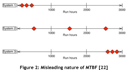
The basic conceptual definition of MTBF necessitates an allowable constant failure rate. Hockley [17] and Mitchell [18] point out that this has translated into the firm belief that random failures are inevitable during the life cycle of equipment. Hockley and Appleton [19] go further, and state that the indiscriminate use of MTBF and the maintenance philosophy associated with it has led to an underlying perception in the belief in and acceptance of failure. This in turn has led to lethargy when it comes to understanding when and why failure takes place in the first place. MTBF can also be misleading for non-constant hazard rates [20]. This misleading nature of MTBF and its ability to hide information can be seen in Figure 2, where three systems with their failures over the same time period are shown. System 1 is characterised by three early failures, System 2 displays three failures at equal intervals over the time period, and System 3 has three late failures. However, all three systems, with their vastly differing behaviour, have exactly the same MTBF of 1,000 hours - illustrating the fact that the MTBF hides detailed information. It should be noted that if the frequency were changed in Figure 2 and were kept up to date over time, the three systems shown below would show different MTBFs. However this is seldom done in industry.

 

 

MTBF can be described as catering to the 'one number syndrome', and it is actually a gross over-simplification of the problem. The use and application of MTBF as a reliability metric is deceptive and frequently mishandled, causing ambiguity and wasted effort [21].

Relf [12] points out that the MTBF methodology conveys the impression that there is a certain 'allowable' level of failure that can be classified as random. It can also be seen that MTBF accepts failure and cannot be accurately forecast and avoided [23]; it therefore has a negative impact, as it induces unscheduled maintenance activities that, in turn, negatively impact the total life operating cost of the system. Trindade and Nathan [22] very clearly state that there is a need for a better reliability metric that accounts for trends in failure data.

It can be seen by the definition and use of the reliability metric MTBF that a number of inherent and fundamental problems occur with it. The MTBF presumes that failure is inevitable, and thus creates the general assumption that there is no point in striving for the ultimate goal of reliability excellence. This has necessitated a fundamental shift in the way reliability is measured, and has led to the development of a new reliability metric from within the aviation sector that attempts to address the problems identified with the MTBF maintenance interval metric.

 

4 MAINTENANCE FREE OPERATING PERIOD (MFOP) - DEVELOPMENTS FROM AVIATION MAINTENANCE

The aviation maintenance industry is at the forefront of maintenance technology and practices, due to the innate risks with which it operates. One example is the reliability centred maintenance (RCM) methodology, which originated in the aviation sector and has since found wide acceptance in a vast number of other industries. Another development stemming from the aviation sector is a new reliability metric called the maintenance free operating period (MFOP), defined to address some of the inherent problems associated with the application of MTBF.

4.1 Maintenance free operating period (MFOP)

The maintenance free operating period (MFOP) is the aviation sector's proposed solution to the problems found when applying MTBF to specify reliability. MFOP is defined by a number of authors ([18],[21],[23],[24],[25]) as:

A period of operation during which the system must be able to carry out all of its assigned missions without any maintenance action and without the operator being restricted in any way due to systems faults or limitation.

It should be noted that during an MFOP, the system in question is allowed to undergo any planned minimal maintenance, such as with consumables ([18],[24],[26]). The MFOP principle encourages the use of fault-tolerant, redundant, and re-configurable systems [21]. This is seen because redundant components are allowed to fail during the MFOP without forcing any unscheduled or corrective maintenance. In effect, Manzini et al. [25] state that under an ideal MFOP policy, corrective maintenance needs to be bypassed.

Another important term is the maintenance recovery period (MRP). This stems from the fact that major preventive maintenance should only be carried out in previously arranged periods. A MRP is defined as follows [21],[27]: A period of a certain specified duration dependent on the maintenance task that is required. The requirement that periodic maintenance tasks be of different durations for minor and major activities would not change. It can therefore be seen that the length of the MRP is flexible and dependent on the previous and the next MFOP, as well as on the extent of maintenance required.

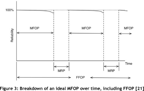
A final term that is generally relevant is the failure-free operating period (FFOP), defined by Brown and Hockley [21] and Mitchell [18] as "A period during which the equipment shall operate without failure, however, faults and maintenance both planned and unplanned are permissible, i.e. all planned operations and cycles are completed unchanged". Figure 3 shows an ideal MFOP cycle including FFOP. Each MFOP is a finite period of operation that is followed by a MRP of specified duration.

 

 

4.2 Explanation of MFOP - the paradigm shift

For a better understanding of the approach, a brief analysis of the fundamental concept of MFOP is given here. As previously stated, MTBF by definition accepts failure, thus inducing corrective maintenance activities. This in turn has a negative impact on the total life operating cost. Taking this into account, it would be advantageous to be able to guarantee a certain MFOP; this would decrease corrective or unscheduled maintenance, thereby reducing the total life cycle operating cost of the system. In this regard, MFOP amounts to a maintenance philosophy that builds on the operational requisite of needing periods of guaranteed availability and reliability.

Long [23] mentions that the MFOP methodology drives change in three areas: design, operation, and maintenance planning. Three main pillars are used by MFOP to achieve success in an operating environment with minimal maintenance: failure anticipation, avoidance, and maintenance delay. A key contrast between MFOP and MTBF is the fact that MFOP assumes, from the beginning, that success is attainable and that the probability of success can be accurately forecast. MFOP specifies customers' needs in unambiguous terms [21]. Another point by Hockley [17] is that, as MFOP attempts drastically to reduce corrective maintenance and the associated costs, this would substantially increase a company's asset effectiveness and lower the supportability costs of their assets. Figure 4 shows some motivators for the application of MFOP as a reliability metric. Included in Figure 4, Brown and Hockley [21] make the point that by applying the MFOP methodology, maintenance needs would be more accurately known, thus decreasing the logistical footprint and spares consumption. These points about the respective approaches of MTBF and MFOP are summarised in Table 1.

 

 

By applying the MFOP concept, reliability of equipment would be improved and enhanced, and more focused improvements could be made. This is because the philosophy forces operators to know the equipment, making them more likely to identify the true causes of failure. Khan [28] states that the greatest competitive advantage in today's global environment is equipment reliability. Applying MFOP instead of MTBF would go a long way to achieving this.

 

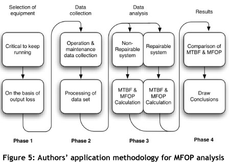
5 METHODOLOLGY FOR ANALYSING SYSTEMS

A methodology to analyse the MFOP performance of systems is presented in this section. The authors have synthesised it from various sources. An overview is given in Figure 5. It is split into four distinct phases. In Phase 3, data analysis and failure statistics are applied to the data set found in Phase 2. Two different streams are given in Phase 3: one for a non repairable system, the other for a repairable system. The developed methodology is applied later in a case study, discussed in Section 6.

 

 

5.1 Phase 1: Selection of equipment

When equipment is selected for the application of the MFOP methodology, two basic questions should be asked. Is it critical that the equipment be kept running, thus needing minimal interruptions or unplanned maintenance? This decision should be made to minimise the potential output loss of this equipment by reducing, and ultimately eliminating, the need for unplanned maintenance.

Setting system boundaries is also important in this phase. This can depend on the level of detail available in the failure data; if very detailed maintenance data is available, the study can be conducted on a single component level. Horizontally, the system boundaries are dependent on the complexity of the system and of the systems around it.

5.2 Phase 2: Data collection

It is very important that the correct maintenance data is sampled. The maintenance data only needs to be relevant to the system that is chosen for the analysis. Job cards need to be processed to ascertain the root cause failure. Two types of data points are obtainable: the first is a failure, where the system failed completely and the operation had to be stopped; the second is a suspension, or suspended data point, where scheduled maintenance was carried out on the system. A database should be created for the data set found; the preferred software for this purpose would be Microsoft Excel.

5.3 Phase 3: Data analysis

Two types of systems are available within this phase: a non-repairable and a repairable system. A non-repairable system is defined by Ascher and Feingold [30] as a system that is discarded after its first failure at system level. A repairable system is defined by the same author [30] as a system that, after failing to perform one or more of its functions satisfactorily, can be restored fully by any method other than complete replacement. In this paper, systems are generally described as either repairable or non-repairable, based on the properties of the failure data they generate, and on their physical properties. Failure data from a system that is independent and identically distributed is classed as non-repairable, and failure data from a system that displays a trend (increasing or decreasing) is classed as repairable. Even if a system is physically repairable, it can still produce failure data that is independent and identically distributed, and would therefore be classed as non-repairable for the analysis.

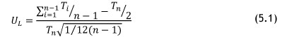
The first step within this phase is to determine whether a trend is present in the data set found in the previous phase. The Laplace trend test is commonly used for this; it tests whether a trend is present in a data set, and thereby determines whether the data follows a homogenous Poisson process (HPP) or a non-homogenous Poisson process (NHPP). If a trend is present in the data, it can be modelled as a repairable system using an NHPP, for which the power law NHPP can be used to model the system. Once the system has been modelled in this way, the MFOP of the system can be computed. The Laplace trend test is shown in Equation 5.1.

The following outcomes are possible from the Laplace test: if U_L ≥ 2 then there is strong evidence for reliability degradation; whereas if U_L < -2 then there is strong evidence for reliability improvement. Between -1 < U_L < 1, there is no evidence of an underlying trend. In the two cases where 2 > U_L > -1 or -1 > U_L > -2, the Laplace test cannot indicate with certainty whether or not a trend is present in the data set; in such a case an alternative trend test such as the Lewis-Robinson test can be applied.

5.3.1 Non-repairable system analysis

As mentioned above, even if the physical system is classified as repairable, it may still behave in a way that yields data that calls for a non-repairable HPP system analysis. This is the case if the Laplace trend test shows that there is no trend present in the data set; the Weibull distribution, shown in Equation 5.2, is then used for this purpose.

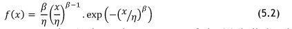
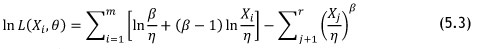
Here β is the shape parameter and η is the scale parameter of the Weibull distribution, with β > 0 and η > 0. To calculate the parameters β and η numerically, the 'maximising the likelihood' method can be applied; this is shown in Equation 5.3.

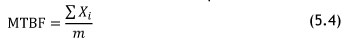
Now that the parameters of the Weibull distribution can be found, the MTBF and MFOP calculations can be performed. The numeric MTBF is found in Equation 5.4.

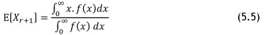
The statistical MTBF can be calculated by Equation 5.5 [31].

MFOP can now be calculated using Equation 5.6 [24]. However, before this is shown, we introduce and define the term 'maintenance free operating period survivability' (MFOPS) as: The probability that the part, subsystem, or system will survive for the duration of the MFOP, given that it was in a state of functioning at the start of the period [24].

Here, Equation 5.6 gives the probability of surviving t_mf units of time, given that the system has already survived t units of time. From these calculations, conclusions can be made about the actual performance of the system that is analysed by comparing the MFOP with the MTBF.

5.3.2 Repairable system analysis

The second possibility of Phase 3 in the methodology is the repairable systems theory. If the Laplace trend test showed that there is an underlying trend in the data set, then the system should be modelled using the power law NHPP shown in Equation 5.7.

In order to estimate the parameters λ and δ of Equation 5.7, the least squares method is used (though this will not be elaborated on in this paper). Now that the system can be modelled using the power law NHPP and the parameters are numerically known, the MTBF and MFOP calculations can be performed. The numeric MTBF is found in Equation 5.8 [31].

The statistical MTBF for a repairable system can be calculated by Equation 5.9 [31], where the system is put back into operation after the last recorded failure, and then the next failure of the system can be predicted.

The calculation of the MFOP of a repairable system can now be performed using Equation 5.10; this equation is derived, as with a non-repairable system, from the reliability function.

Here, T_r is the global time unit of the last known time event, and the parameters λ and δ have been found previously through the least squares method.

 

6 CASE STUDY

The case study conducted in this section applies the MFOP principle to a real-life system found in the mining sector. The case study was conducted through Anglo American Plc, at their subsidiary Anglo Platinum. Data was collected at one of Anglo Platinum's bushveld complex mines in South Africa.

6.1 Chosen system

The system that was chosen to be studied was an arrangement of three cone crushers. These cone crushers are used for secondary crushing operations; the relative position of the crushers within the system is shown in Figure 6.

 

 

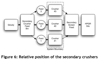
The crushers are pivotal to the smooth operation of the complete system and of the equipment that is situated downstream. They have been found to be susceptible to breakdowns and unscheduled maintenance activities in the past and to hamper the continuous operation of the system. The system boundaries of the crushers are shown in Figure 6. The crushers are analysed individually, and any failure pertaining to one of the crushers is included in the data set.

6.2 Analysis of Crusher 3

Due to the repetitive nature of the analysis for each crusher, only the analysis for Crusher 3 is detailed here, with a summary given at the end. Maintenance and failure data was obtained for the crusher within the period 2010 to 2011; about a year of data was collected, yielding 90 events.

In order to gain a better understanding of the predominant causes of failure, a Pareto analysis was conducted on the data set. The Pareto chart is shown in Figure 7, and shows that the top two causes of failure are the lube system and other/unplanned maintenance. The latter category was data points where the root cause of failure could not be identified unambiguously.

 

 

The Laplace trend test was then applied to the data set from Crusher 3, and found to be U_LCR3 = 1.60. This puts Crusher 3 into the grey area of the Laplace test, meaning that the test cannot conclusively say whether or not a trend is present in the data. The Lewis-Robinson trend test, a modification of the Laplace test, was then applied to the data, and a result of U_LRCR3 = 1.59 was obtained. This is still within the grey area of the test, and therefore provides inconclusive evidence of a trend being present or not. This information is necessary in order to know whether the system should be modelled using an HPP or an NHPP. The data set was then looked over again (a failure versus a cumulative time plot can assist with this). Looking at the inter-arrival times of events, it was assumed that no trend was present in the data, and Crusher 3 would be modelled with the Weibull distribution.

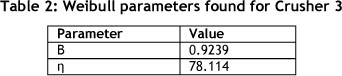
In order numerically to obtain the shape and scale parameters of the Weibull distribution, β, and η respectively, the 'maximising the likelihood method' is used, with the results given in Table 2.

 

 

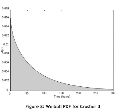
Substituting the parameters found into Equation 6.1 gives the specific Weibull distribution for Crusher 3, shown below.

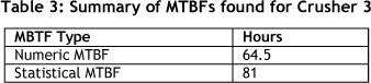
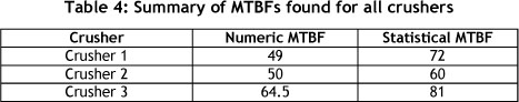
From Equation 6.1, the probability density function (PDF) can be plotted, and is shown in Figure 8. For comparative purposes, the MTBF can be calculated from the data set obtained for Crusher 3. It is possible to calculate two different MTBFs: a numeric MTBF, widely used in industry; and a statistical MTBF calculated with the aid of failure statistics. The results are summarised in Table 3.

 

 

 

As the β and η parameters of the Weibull distribution are now known for Crusher 3, MFOP calculations can be done. Equation 5.6 is used to determine the MFOP and MFOPS for Crusher 3. The plot of the MFOP length against the probability of achievement, MFOPS, is shown in Figure 9 below.

 

 

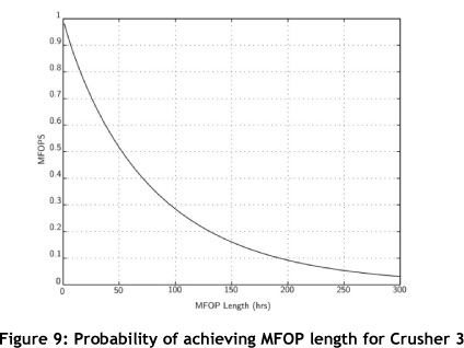
It can be seen from Figure 9 that Crusher 3 does not provide a particularly high MFOP at a high probability of achievement, MFOPS. Comparing the found numeric MTBF value for Crusher 3 of 65 hours with the same length MFOP, it is seen that Crusher 3 has only about a 44 per cent chance of completing that period without requiring any unscheduled maintenance actions. In a 24-hour MFOP, which is relatively easy to comprehend, it can be seen that Crusher 3 has a 71 per cent chance of completing a full day without requiring unscheduled maintenance actions.

A hypothetical case was set up to demonstrate the MFOP principle more clearly. This is done to illustrate how MFOP can be used to create tangible and perceivable reliability targets, expressed in simple percentages. The hypothetical case consisted of the removal of the top two failure cases shown in the Pareto chart in Figure 7. Here the categories 'lube system' and 'other/unscheduled' maintenance were removed from the data set and a new data set was formed. This new data set was then analysed, again using the same methodology. The shape and scale parameters were found, and MFOP calculations were performed on the hypothetical Crusher 3. Figure 10 shows a plot of the MFOP performance for both the current crusher and the hypothetical crusher.

 

 

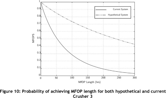
Comparing the two systems, a vast difference is seen in the MFOPS at a certain MFOP length. The hypothetical system is much more reliable than the current system, taking the previously established MTBF of 65 hours. Crusher 3 has a 44 per cent chance of achieving this, while the hypothetical crusher has an 82 per cent chance - a sizable improvement. A complete overview of all three crushers is given in Figure 11.

 

 

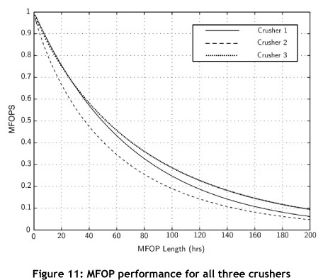
Comparing the MTBFs and MFOPs found for all crushers, shown in Table 4 and Figure 11 respectively, a number of observations can be made. Immediately noticeable is that Crusher 1 and Crusher 2 have an MTBF that is virtually the same; however, their reliability characteristics are vastly different. Looking at MFOP length in Figure 11 (which is equal to that of the shared MTBF of both crushers), it can be seen that at exactly the same MFOP of 50 hours, Crusher 1 has an MFOPS of 50 per cent and Crusher 2 an MFOPS of only 40 per cent. This illustrates the vastly different reality of the crushers' performances, and shows how MFOP provides a more 'complete' picture. Another point to make is that for reliability performance, Crushers 1 and 3 are very similar for about the first 60 hours of operation.

 

 

7 CONCLUSION

The aviation industry has come up with a new reliability metric that addresses the intrinsic issues found when using the MTBF. This new maintenance interval metric is called MFOP. The methodology developed and applied in a mining specific case study enable a number of conclusions to be drawn.

It can be seen that MTBF caters for the 'one number syndrome', oversimplifying the problem that it attempts to address. Using MTBF to describe the reliability of a system creates a certain intellectual laziness. MTBF, by definition, makes the absolute presumption that failure is inevitable, and therefore does not create or foster a culture of excellence or improvement; on the contrary, it yields mediocrity, as it assumes failure.

Analysis of the case study showed that the numeric MTBFs found for the crushers described them in a limited fashion; they did indeed indicate that the system seems unreliable, but only provided a very limited one dimensional view. The MTBF described two of the three crushers as having the same reliability characteristics, even though their reliability was different; MFOP exposed the difference more accurately. A number of other authors have shown that the ethos of MFOP assumes that unscheduled maintenance or failures should not be accepted, but should be minimised as far as possible; and that success is attainable, in direct contrast with the approach of MTBF. The MFOP school of thought demands that reliability management establish and strive for certain time intervals that do not require intervention, because the system can be trusted without being 'touched' to survive the mission; MFOP thus enables better reliability target setting. The results of the case study were presented to Anglo American management, engendering very positive feedback and interest.

An MFOP reliability target is far more tangible and perceivable than an MTBF target. This should enable maintenance engineers to perform more focused maintenance, as reliability targets can now be visually tracked. MFOP is a far more appropriate school of thought and realistic reliability metric to assess the reliability of physical assets.

 

NOMENCLATURE

β Shape parameter for the Weibull distribution

η Scale parameter for the Weibull distribution

Λ, δ Parameters required for the Power Law NHPP

r Total number of observed events

m Total number of observed failures

x Continuous time

X Discrete event time measured in local time

T Discrete event time measured in global time

E[] Expected value

U_L Laplace trend test

x_mf Length of MFOP for non-repairable systems

t_mf Length of MFOP for repairable systems

 

REFERENCES

[1] Heng, A., Zhang, S., Tan, A. & Mathew, J. 2009. Rotating machinery prognostics: State of the art, challenges and opportunities. Mechanical Systems and Signal Processing, 23(3), pp. 724-739.         [ Links ]

[2] Mobley, R. 2002. An introduction to predictive maintenance. Butterworth-Heinemann.         [ Links ]

[3] Vanier, D. 2001. Asset management a to z. NRCC/CPWA/IPWEA Seminar, pp. 1-16.         [ Links ]

[4] Federal Highway Administration. 1999. Asset management primer. Federal Highways Administration. Washington, D.C.         [ Links ]

[5] Hastings, N.A.J. 2010. Physical asset management. Springer-Verlag, London.         [ Links ]

[6] Amadi-Echendu, J., Willett, R., Brown, K., Hope, T., Lee, J., Mathew, J., Vyas, N. & Yang, B. 2010. What is engineering asset management? Definitions, concepts and scope of engineering asset management, pp. 3-16. Proceedings 2nd World Congress on Engineering Asset Management and the 4th International Conference on Condition Monitoring, pages pp. 116-129, Harrogate, United Kingdom.         [ Links ]

[7] Amadi-Echendu, J. 2004. Managing physical assets is a paradigm shift from maintenance. Engineering Management Conference, 3, pp. 1156-1160.         [ Links ]

[8] Woodhouse, J. 2003. Asset management: Concepts & practices. The Woodhouse Partnership.         [ Links ]

[9] British Standards Institution. 2008. PAS 55: Asset management. British Standards Institution. Technical Report.         [ Links ]

[10] Wessels, W. 2012. Design-for-mechanical reliability to risk of failure. RMS Partnership: A Newsletter for Professionals.         [ Links ]

[11] Krellis, O. & Singleton, T. 1998. Mine maintenance - The cost of operation. Coal 1998: Coal Operators' Conference, pp. 91-90.         [ Links ]

[12] Relf, M. 1999. Maintenance-free operating periods - The designer's challenge. Quality and Reliability Engineering International, 15, pp. 111-116.         [ Links ]

[13] Cambell, J., Jardine, A. & McGlynn, J. 2011. Asset management excellance: Optimizing equipment from a life-cycle perspective. 2^nd edition, CRC Press.         [ Links ]

[14] Van der Lei, T., Herder, P. & Wijnia, Y. 2011. Asset management: The state of the art in Europe from a life cycle perspective. Springer Verlag.         [ Links ]

[15] Smith, D. 2005. Reliabilty, maintainability and risk: Practical methods for engineers. 7^th edition, Butterworth-Heinemann.         [ Links ]

[16] U.S. Department of Defense. 1980. MIL-STD-785: Reliability program for systems and equipment development and production. Technical Report. Washington, D.C.         [ Links ]

[17] Hockley, C. 1998. Design for success. Journal of Aerospace Engineering, 212(6), p. 371.         [ Links ]

[18] Mitchell, P. 2000. What the customer wants. Maintenance-free and failure-free operating periods to improve overall system availabilty and reliabilty. DTIC Document.         [ Links ]

[19] Hockley, C. & Appleton, D. 1997. Setting the requirements for the Royal Air Force's next generation aircraft. IEEE, Reliabiity and Maintainability Symposium, pp. 44-49.         [ Links ]

[20] Todinov, M. 2003. Minimum failure-free operating intervals associated with random failures of non-repairable components. Computers & Industrial Engineering, 45(3), pp. 475-491.         [ Links ]

[21] Brown, M. & Hockley, C. 2001. Cost of specifying maintenance/failure free operating periods for the Royal Air Force aircraft. IEEE, Reliability and Maintainability Symposium, pp. 425-432.         [ Links ]

[22] Trindade, D. & Nathan, S. 2006. Statistical analysis of field data for repairable systems. Reliability and Maintainability Symposium.         [ Links ]

[23] Long, J., Shenoi, R. & Jiang, W. 2009. A reliability-centred maintenance strategy based on maintenance-free operating period philosophy and total lifetime operating cost anaylsis. Journal of Aerospace Engineering, 223, p. 771.         [ Links ]

[24] Dinesh Kumar, U., Knezevic, J. & Crocker, J. 1999. Maintenance free operating period - An alternative measure to MTBF and failure rate for specifying reliability? Reliability Engineering & System Safety, 64, pp. 127-131.         [ Links ]

[25] Manzini, R., Regattieri, A., Pham, H. & Ferrari, E. 2009. Maintenance for industrial systems. Springer Verlag.         [ Links ]

[26] Kumar, U. 1999. New trends in aircraft reliability and maintenance measures. Journal of Quality in Maintenance Engineering, 4, pp. 66-75.         [ Links ]

[27] Dinesh Kumar, U., Crocker, J., Chitra, T. & Saranga, H. 2006. Reliability and six sigma. Springer Verlag.         [ Links ]

[28] Khan, F. 2001. Equipment reliability: A life cycle approach. Engineering Management Journal, 11(3), pp. 127-135.         [ Links ]

[29] Chew, S. 2010. System reliability modelling for phased missions with maintenance free operating periods. PhD thesis, Loughborough University, Leicestershire, England.         [ Links ]

[30] Ascher, H.& Feingold, H. 1984. Repairable systems reliability: Modeling, inference, and misconceptions and their causes. M. Dekker Publishers.         [ Links ]

[31] Vlok, P.J. 2011. Introduction to practical statistical anaylsis of failure time data: Long term cost optimization and residual life estimation. Course notes.         [ Links ]