


Services on Demand
Article
 English (pdf)
 Article in xml format
 Article references
Indicators

Related links
-
 Cited by Google
 -
 Similars in Google
Share

 Permalink
South African Journal of Industrial Engineering
On-line version ISSN 2224-7890
Print version ISSN 1012-277X
S. Afr. J. Ind. Eng. vol.24 n.2 Pretoria Jan. 2013
CASE STUDIES
Managing bottlenecks in manual automobile assembly systems using discrete event simulation#
M. DewaI, *; L. ChidzuuII
IDepartment of Industrial Engineering Faculty of Engineering and the Built Environment Durban University of Technology, South Africa. mendond@dut.ac.za
IIDepartment of Industrial Engineering Faculty of Engineering and the Built Environment Durban University of Technology, South Africa. libertychidzuu@gmail.com
ABSTRACT
Batch model lines are quite handy when the demand for each product is moderate. However, they are characterised by high work-in-progress inventories, lost production time when changing over models, and reduced flexibility when it comes to altering production rates as product demand changes. On the other hand, mixed model lines can offer reduced work-in-progress inventory and increased flexibility. The object of this paper is to illustrate that a manual automobile assembling system can be optimised through managing bottlenecks by ensuring high workstation utilisation, reducing queue lengths before stations and reducing station downtime. A case study from the automobile industry is used for data collection. A model is developed through the use of simulation software. The model is then verified and validated before a detailed bottleneck analysis is conducted. An operational strategy is then proposed for optimal bottleneck management. Although the paper focuses on improving automobile assembly systems in batch mode, the methodology can also be applied in single model manual and automated production lines.
OPSOMMING
Lotgrootteproduksielyne kom baie handig te pas wanneer die vraag vir elke produk matig is. Lotgrootteproduksielyne word egter gekenmerk deur hoë werk-in-prosesvoorraad, verlore produksietyd wanneer modelle verander en verlaagde buigsaamheid wanneer dit kom by die verandering van die produksietempo's as produkaanvraag verander. Gemengde modelproduksielyne kan egter verlaagde werk-in-prosesvoorraad en verhoogde buigsaamheid bied. Die doel van hierdie artikel is om te illustreer dat 'n handgedrewe voertuigmonteringsisteem geoptimiseer kan word deur bottelnekke te bestuur deur hoë werkstasie-benutting te verseker, die toulengtes voor werkstasies en werkstasiestilstand te verminder. 'n Gevallestudie uit die motorindustrie word gebruik vir data-insameling. 'n Model is ontwikkel deur die gebruik van simulasiesagteware. Die model word dan geverifieer en bekragtig voordat 'n gedetailleerde bottelnekanalise gedoen word. 'n Operasionele strategie word vervolgens voorgestel vir optimale bottelnekbestuur. Hoewel die artikel fokus op die verbetering van motormonteersisteme wat in lotgroottes bedryf word, kan die metode ook toegepas word op 'n enkelmodel hand- en outomatiese produksielyne.
1. INTRODUCTION
Assembly lines can be classified into single-model, batch-model, and mixed-model lines. In a batch-model assembly system, a few product models are produced in batches, with one product at a time on the same line, and a certain amount of changeover time is allotted to ready the line for the production of another model [1]. In recent decades, the need for more versatile and flexible production has forced assembly line production systems to change from fixed assembly lines to mixed-model assembly lines, where the output products are variations of the same base product and only differ in specific customisable attributes [2]. Considering mixed-model manual automobile assembly systems, setup times between models can be reduced enough to be ignored, so that intermixed model sequences can be assembled on the same line.
A procedure is needed to determine a particular configuration for the products to be produced on the line that will not only minimise the balance delay or number of workstations, but also satisfy other conflicting criteria such as production rate, variety, minimum distance moved, division of labour, and quality [1]. The key input to a line balancing problem is accurate standard time derived from a time study or from any other work measurement technique.
For a traditional direct time study, a time-study analyst divides a job that usually takes a long time into basic tasks that are easier to measure and analyse; and then the analyst observes a qualified person using the best method to perform the job [3]. The time standard is the time required by a skilled operator, working at a normal pace, to perform a specific task using a prescribed method, allowing time for personal needs, fatigue, and delays. It can be used for a work assignment, for evaluating the numbers of workers, the type and capacity of machines, the overall productivity, the total cost for product manufacturing, and so on.
Bottlenecks for one product are not automatically bottlenecks for other products in the same manufacturing line. This is due to variations in the processing time for the different products on different machines [4]. An important trend in the queuing theory literature that can be used in bottleneck analysis is the development of laws that connect the system content and customer delay. The most well-known result is Little's law, which is valid for any arrival process, service process, or scheduling discipline, but only deals with the first moments of system content and delay [5]. According to Masood [6], increased throughput and higher machine utilisation in an automotive plant can be achieved by managing bottlenecks through line balancing. Das [7] discusses the conceptual overview of a simulation methodology to evaluate assembly line balancing with variable operation times based on the next-event analysis. Pourbabai [8] proposes a methodology for the design of a flexible assembly line system while controlling the bottleneck problem. Plenert [9] demonstrates how geometric programming can be used to solve an industrial bottleneck with an unlimited number of products and multiple constraints. Wang [10] proved that a data-driven approach can enable the modelling and simulation of a complex assembly plant in a real-time fashion, and thus effectively improve the responsiveness and flexibility of the production line.
The aim of this paper is to use a discrete-event simulation package to illustrate that bottlenecks can be managed by ensuring high workstation utilisation, reducing queue lengths before stations, and reducing station downtime. The paper begins with background information on the case in point. The second section of the paper comprises the work approach from time studies to quantitative analysis of mixed-model assembly lines. A simulation model is then developed using Showflow simulation software. The model is verified and validated using information derived from actual historical data. A detailed bottleneck analysis is then conducted, after which decisions are made for optimal bottleneck management. The paper also demonstrates that simulation can be a tool for determining the makespan for specified vehicle demand so that due dates for orders from customers are met.
2. BACKGROUND
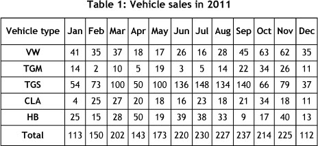
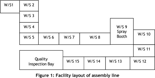
The assembly line of the case in point produces seven truck models and six bus models, operating in batch mode. A summary of vehicles assembled in 2011 is shown in Table 1. The assembly plant is made up of 15 workstations (WS), divided into three zones with different supervisors and group leaders. Zone 1 includes WS 1 to WS 6, zone 2 includes WS 7 to WS 11, and zone 3 WS 12 to WS 15. There is a quality inspection bay at the end of the assembly line where all vehicles are inspected for faults. All detected faults are noted in the vehicle's protocol book.
In collective working, as practised in the final assembly of motor vehicles, several operators work on one or more products at a workstation designed for group work. The product is released from this workstation when all operators have completed their work. It is then replaced by another product. Correctly designed, this method of working provides the opportunity to reduce time losses caused by variations in work pace, imbalances in the division of labour, and product variant differences, or so-called balance loss [11]. The case in point operates its fifteen-station assembly system in an asynchronous mode, and there are no storage buffers between the stations owing to the facility's space constraints and the firm's policy on minimising work-in-progress inventory. For the sake of job enrichment, workers are dedicated to particular assembly stations and are trained to perform a restricted set of assigned tasks. On the 15 assembly plant workstations, bottlenecks keep on migrating due to variation in station cycle times and other system dynamics.
3. METHODOLOGY
This section describes the approach we used to address the problem of poor bottleneck management. The following steps were proposed and followed:
- Conduct time studies and establish standard times
- Develop the simulation model
- Verify and validate the simulation model
- Quantitatively analyse the mixed model assembly lines
- Conduct bottleneck analysis
- Make decisions to optimise bottleneck management
4. DATA COLLECTION
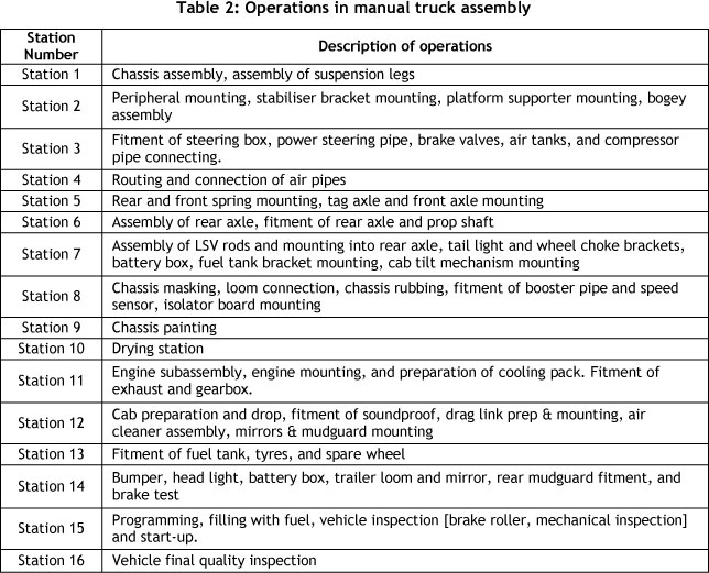
The data required for simulation was collected through direct observation of the assembly line. The standard times had been updated four years previously, and there had been changes within the company in production, in the variability in material or parts used to assemble the vehicles, and in the methods used. State-of-the-art tooling that takes much less time to perform tasks was now available, and new models had been introduced to the assembly line. It was against this backdrop that we decided to conduct time studies. We observed the assembly operators, and recorded the operation sequences and potential break points on the standard operations sheet. Table 2 shows a summary of typical operations during the assembly of a truck.
We split the operations into elements, and timed the individual elements as many times as was necessary till the end of the operation. Table 3 shows a summary of assembly times for five key vehicle models.

5. SIMULATION MODELLING
5.1 Development of simulation model
In discrete-event simulation (DES), the operation of a system is represented as a chronological sequence of events. Each event occurs at an instant in time and marks a change of state in the system [15]. Input data to the simulation model was extracted directly from the data files of the process control department. The assembly plant facility layout was used as the basis for the layout of the simulation model to enable it to be accurate and realistic. Discrete-event simulation is an experimental approach that is often used; it allows a high level of detail to be modelled since assumptions about buffer space, processing time distributions, or priority dispatching can be modelled [13]. It was assumed that all stations would be available for assembly operations and that the new spray booth had negligible downtime. It is also critical to note that the final vehicle inspection station would not constrain the main assembly line, since the finished vehicle could be moved away from the line and not block station 15. Figure 1 is a schematic diagram of the facility layout of the assembly line that was used for the Showflow model.
The model was coded using trigger language interpreter (TLI). For example, a table for processing times is first created, and a job parameter such as the processing time for the first vehicle model on the first workstation will be coded as elem[product[E,1],1]. TLI was also used to control entry of vehicles into the first workstation - i.e.
if elqueue[E]>1 then elaccept[E]:=false.
5.2 Verification and validation of the simulation model
After building the model, verification and validation were carried out to check the accuracy of the model. The productions' historical data was compared with the simulation data, and showed acceptable accuracy - less than five per cent deviation from real values. The objective of model verification was to ensure that the conceptual model was reflected accurately. Table 4 shows simulation results for a 30-day period for vehicles entering the assembly line hourly, in the sequence VW-HB-TGM-TGS-CLA.
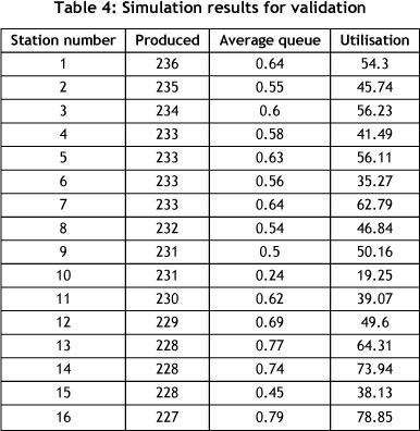
We used the time representation 60 units = 1 minute, 60 minutes = 1 hour, 8 hours = 1 day. The simulation results for vehicles produced are in line with the average monthly sales shown in Table 1 - an indication that the lumped model input/output relations accurately map those of the real system [16].
6. RESULTS AND DISCUSSION
6.1 Quantitative analysis of mixed model assembly lines
Many factors affect the dynamic behaviour of work flow in manual assembly systems. The average utilisation and the number of tasks per job obviously affect average flowtime and work-in-process inventory levels. It is also intuitive, based on elementary queuing theory, that the variance of job inter-arrival times and the variance of processing times on individual machines affect flowtimes [12]. Basic terminology about queuing systems for both infinite and finite sources has been adequately covered by Stevenson [13]. This includes the characteristics of waiting lines, arrival and service patterns, queue discipline, and measures of waiting line performance. The case scenario is an infinite source situation, single-channel, multi-phase system. The inter-arrival times are considered to be constant, and vehicles are assembled on a first-come, first-served basis.
According to Little's law, for a stable system the average number of vehicles in the assembly line Ls is equal to the average vehicle arrival rate λ, multiplied by the average time spent by a vehicle in the assembly line Ws [13]. That is:

System utilisation ρ is computed as:

where λ = vehicle arrival rate at station 1; M = number of servers; µ = service rate/ server. The average time a vehicle is in the assembly line Ws is given as:

where Wq = the average time a vehicle waits in the queue.
The performance metrics for the manual assembly line, including the average number of vehicles waiting in the line, the average time a vehicle waits in the line, and system utilisation, were used for the bottleneck analysis in Section 3.5, and are based on equations 1, 2, and 3. LsLsLsLsLswas obtained by physically counting the vehicles on the assembly line, and Ws from the desired takt time, which was a function of the demand.
The quantitative analysis of mixed model assembly lines used in the paper was derived from Groover [14]. The number of workers w is computed as:

where WL = workload to be accomplished by the workers in the scheduled time period (min/hr); AT = available time per worker (min/hr per worker), where

where Rpj = production rate of model j (vehicles/hr) and Twcj = work content of model j (min/vehicle). p = number of vehicle models to be produced during the period, and j is used to identify the model.
Rpj is computed as a function of annual demand, and Da for the vehicle models shown in Table 1, using equation 6.

where sw is the number of shifts per day and Hsh is the number of working hours per shift. Equations 4, 5, and 6 were used to determine the number of workers required, as shown in the last column of Table 3.
For instance, for station 1, using eight hours per shift, one shift per day, 50 weeks per year, and annual demand values from Table 1, the hourly assembly rate is 0.36 for VW, 0.42 for TGM, 2.79 for TGS, 0.6 for CLA, and 0.81 for HB Bus. This gives an average production rate of one vehicle/hr for the assembly line.
To compute the available time per worker (WL), the work content of each model is obtained from the first row of Table 3, and the average production rate of the line is one vehicle/hr, to give WL = 166 min/hr.
Assume AT = 60 minutes as the available time per hour, and factor in an efficiency of 80 per cent; this results in 48 minutes being available per hour. Computing the number of workers w will give 3.45, which we rounded up to 4 workers.
In mixed model assembly line balancing, the objective function can be expressed as:

This constraint was crucial in optimally assigning the workers to stations to minimise worker idling or maximise worker labour utilisation. The decisions about optimal bottleneck management in Section 6.3 are based on this constraint.
6.2 Bottleneck analysis
The model was simulated for a 30-day period, with five vehicle models entering the assembly line while different parameters were varied. A low value of every 15 minutes for the rate of vehicle entry to the first station was chosen so that it would not bottleneck the process. Bottleneck analysis was then conducted by analysing the effect of vehicle sequence, batch sizes, individual vehicle models, subassemblies, and downtime on the desired performance metrics.
6.2.1 Analysis of effect of vehicle sequencing
Bottleneck analysis was begun by simulating 25 combinations of assembly sequences for the five vehicle models to find a better sequence than VW-HB-TGM-TGS-CLA, which was being used, based on the shortest total processing time rule. Figure 2 shows the results for the comparison of station waiting times for five assembly sequences (sequences for A, B, C, D, and E are shown in Table 5).
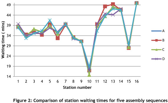
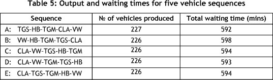
The sequence TGS-HB-TGM-CLA-VW outperformed other sequences in the number of vehicles produced, the total waiting time, and the average queues of vehicles at stations, as shown in Table 5. The results also demonstrated slight disparities in station utilisation. Analysis of the status diagram of the simulation results indicated a high frequency of blockages at stations 10 and 6, while stations 2 and 4 were the most idle ones.
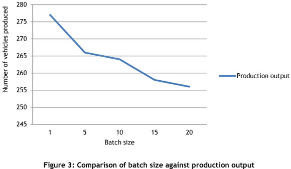
6.2.2 Analysis of effect of batch sizes
The effect of assembling a single-unit batch sizes, compared with batch sizes of up to a maximum of 20 vehicles, was then analysed using the sequence TGS-HB-TGM-CLA-VW. It found that the single unit batch size was superior for the number of vehicles produced, for higher station utilisation, and for lower average queue lengths. Figure 3 shows the effect of increasing the batch size on production output.
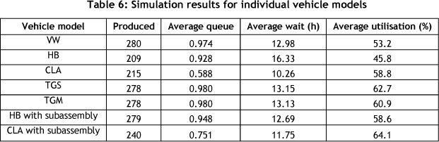
6.2.3 Analysis of individual vehicle models
The individual vehicle models were then simulated to identify precisely the effects of individual models and the actual locations of bottleneck stations; these results are shown in Table 6. Analysis of simulation results revealed that the CLA truck and HB bus were the most problematic, owing to the complexity of the assembly activities executed. The results from the simulation model demonstrate that the first station was a bottleneck when assembling the CLA truck, as it had the longest waiting time for vehicles in the queue when using the FIFO queue discipline [17].The main reason for this bottleneck was that the operators have to assemble the cross members and fit them at the same time. The average waiting time of the assembly line at station 14 was also adversely increased by the HB bus, because mounting operations of the bumper, head light, battery box, trailer loom, mirror, and rear mudguards, as well as brake tests, are undertaken by six workers.
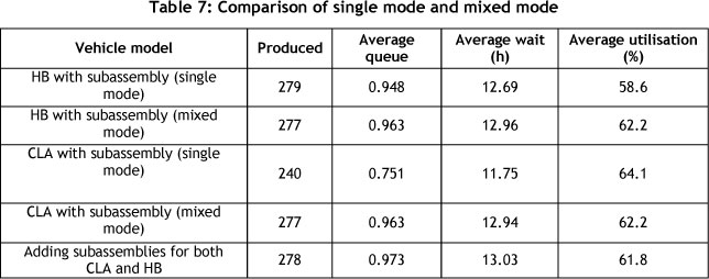
6.2.4 Analysis of the effect of a subassembly
When demand increased, there was a need to reduce the takt time from one hour to 50 minutes. A subassembly was introduced at station 14 when assembling the HB bus, and at station 1 when assembling the CLA truck, to reduce the takt time. The results from the simulation model shown in Table 7 were used to analyse the effect of subassemblies on both single mode and mixed mode. The results show that introducing a subassembly for the HB bus results in an increase in average utilisation of the assembly line compared with the single mode, although the single mode will produce two more vehicles during the simulated 30-day period.
Conversely, for the CLA truck using the same scenario, the average line use decreases while the total number of vehicles produced increases. Adding subassemblies for both CLA and HB under the same production run yields one more vehicle for the 30-day period at a slightly lower line utilisation of 61.8 per cent.
6.2.5 Analysis of the effect of downtime
Simulation of the model was also conducted with a special focus on station 9, assuming four per cent downtime on the painting station and exponential distribution of the runtime. The results show a production loss of about 10 vehicles for every 30 working days.
The stop-time simulation settings were also varied to determine the actual number of vehicles that could be produced to meet particular due dates for orders from customers, if the vehicles were assembled in mixed mode. For example, 68 vehicles could be produced in 10 days, 108 vehicles in 15 days, 148 vehicles in 20 days, and 227 vehicles in 30 days.
6.3 Decision-making for optimal bottleneck management
Analysing the vehicle sequencing revealed that, if there is demand for all five vehicle models, the best sequence would be TGS-HB-TGM-CLA-VW. It is advisable to ensure that the model with the longest total assembly time is followed by the one with the shortest, the one with the second longest is followed by the one with the second shortest, and the one with average assembly time is in the middle. This helps to reduce the throughput time and effectively utilises the workers. Bottlenecks can also be effectively managed by assembling the vehicles in single-unit batch sizes.
In manual assembly, the time the assemblers spend fetching parts often constitutes a considerable portion of each work cycle, thus impacting substantially on assembly cost. Consequently, the use of kitting, which can reduce the time for fetching parts, is an important aspect to consider to reduce vehicle queues [18].
The recommendation would be to reduce the number of operators at a work station if the labour utilisation at a station is too low. Conversely, if the labour utilisation at a particular station is too high and constrains the whole line, the number of operators working on this work station should be increased. If the labour utilisation is just below the required target, the recommendation would be to move functions from another work station to this work station. If the labour utilisation is just above the required target, functions should be moved from this work station to another station that has the capacity to work on the functions.
Using this logic, it was imperative to introduce the cross member sub-assembly next to station 1 when assembling the CLA truck; this resulted in a reduction in assembly time from 64 minutes to 50 minutes. A battery box sub-assembly at station 3 was also introduced for the CLA truck. An additional worker will be required at station 14 when processing an HB bus, since the functions cannot be moved to another station.
It was also highly recommended to use a variable takt time that would be a function of the monthly demand. When demand increases, takt time should decrease up to 40 minutes. This calls for more resources at stations 2 and 3 for the CLA, station 5 for CLA and VW, station 7 for CLA, station 12 for VW and CLA, and station 14 for TGM, CLA, and VW. It is also critical to institute a reliability-centred maintenance programme that ensures an optimal preventive maintenance scheme, especially for station 9.
7. CONCLUSION
The case study demonstrates a methodology that integrates queuing theory and simulation for optimal bottleneck management. An optimal sequence for mixed mode production can be determined through simulation. The simulation experiments revealed that the proposed mixed-model approach for manual automobile systems at the case in point outperforms the conventional batch production mode. It demonstrated that bottlenecks migrate when there is a product changeover on the assembly line. The purpose of bottleneck analysis was to find the bottleneck in a production line. Different vehicles are made on the line, with the same routing but with varying processing times. This simulation model clearly demonstrated that the machine with the highest degree of utilisation does not necessarily have to be the bottleneck. When the model was simulated, one could trace the bottleneck by finding out which machine was most blocked. The machine next to this one was the bottleneck.
The paper also demonstrated that simulation can be used as a tool to determine the due dates for orders from customers through varying stop-time simulation settings. Efforts to improve manual automobile assembly lines should begin with the required takt time, and then find ways to achieve it using an optimal number of workers.
Future research will be directed towards automating the manual automobile systems to reduce makespan and improve productivity. The development of heuristics for sequencing mixed models for manual assembly systems is also an area for future research.
REFERENCES
[1] Kabir, M.A. & Mario, T.T. 1995. Batch-model assembly line balancing: A multiattribute decision making approach, International Journal of Production Economics, 41(1), pp 193-201. [ Links ]
[2] Battini, D., Persona, A., Sgarbossa, F. & Faccio, M. 2009. Balancing-sequencing procedure for a mixed model assembly system in case of finite buffer capacity, International Journal of Advanced Manufacturing Technology, 44(1), pp 345-359. [ Links ]
[3] Novoa, C.M. 2009. Bootstrap methods for analyzing time studies and input data for simulations, International Journal of Productivity and Performance Management, 58 (5), pp 460-479. [ Links ]
[4] Arne, I., Torbjrn, Y. & Gunnar S.B. 2005. Reducing bottle-necks in a manufacturing system with automatic data collection and discrete-event simulation, Journal of Manufacturing Technology Management, 16(6), pp 615-628. [ Links ]
[5] Gao, P., Wittevrongel, S., Laevens, K., De Vleeschauwer, D. & Bruneel, H. 2010. Distributional Little's law for queues with heterogeneous server interruptions, Electronics Letters, 46(11), pp 763-764. [ Links ]
[6] Masood, S. 2006. Line balancing and simulation of an automated production transfer line, Assembly Automation, 26(1), pp 69-74. [ Links ]
[7] Das, B., Sanchez-Rivas, J., Garcia-Diaz, A. & MacDonald, C.A. 2010. A computer simulation approach to evaluating assembly line balancing with variable operation times, Journal of Manufacturing Technology Management, 21(7), pp 872-887. [ Links ]
[8] Pourbabai, B. 1994. Design of a flexible assembly line to control the bottleneck, Computer Integrated Manufacturing Systems, 7(2), pp 122-133. [ Links ]
[9] Plenert, G.J. 1993. Generalized model for solving constrained bottlenecks, Journal of Manufacturing Systems, 12(6), pp 506-513. [ Links ]
[10] Wang, J., Chang, Q. Xiao, G., Wang, N., Li, S. 2011. Data driven production modeling and simulation of complex automobile general assembly plant, Computers in Industry, 62(7), pp 765-775. [ Links ]
[11] Engstrom, T. & Medbo, L. 1994. Intra-group work patterns in final assembly of motor vehicles, International Journal of Operations & Production Management, 14(3), pp 101-113. [ Links ]
[12] Enns, S.T. 1998. Work flow analysis using queuing decomposition models, Computers & Industrial Engineering, 34(2), pp 371-383. [ Links ]
[13] William J.S. 2007. Operations management, 9th edition, McGraw-Hill Irwin. [ Links ]
[14] Mikell, P.G. 2001. Automation, production systems and computer integrated manufacturing, 2nd edition, Prentice Hall. [ Links ]
[15] Robinson, S. 2004. Simulation - The practice of model development and use, Wiley. [ Links ]
[16] Pidd, M. 2004. Computer simulation in management science, 5th edition, John Wiley & Sons, Ltd. [ Links ]
[17] Incontrol Enterprise Dynamics. 2001. Showflow simulation software, Incontrol Simulation Software. [ Links ]
[18] Hanson, R., Medbo, L. & Medbo, P. 2012. Assembly station design: A quantitative comparison of the effects of kitting and continuous supply, Journal of Manufacturing Technology Management, 23(3), pp 315-327. [ Links ]
# This is an extended version of a paper presented at the 2012 CIE conference
* Corresponding author

