GENERAL ARTICLES

 

Economic design of VSI GCCC charts for correlated samples from high-yield processes

 

 

Y.K. Chen^{I, *}; H.C. Liao^II; C.T. Chen^III

^IDepartment of Distribution Management National Taichung University of Science and Technology, Taiwan. ykchen@nutc.edu.tw
^IIHealth Services Administration Chung-Shan Medical University, Taiwan. hcliao@mercury.csmu.edu.tw
^IIIDepartment of Distribution Management National Taichung University of Science and Technology, Taiwan. chen.chihteng@gmail.com

 

 

---

ABSTRACT

Generalised cumulative count of conforming (GCCC) charts have been proposed for monitoring a high-yield process that allows the items to be inspected sample by sample and not according to the production order. Recent study has shown that the GCCC chart with a variable sampling interval (VSI) is superior to the traditional one with a fixed sampling interval (FSI) because of the additional flexibility of sampling interval it offers. However, the VSI chart is still costly when used for the prevention of defective products. This paper presents an economic model for the design problem of the VSI GCCC chart, taking into account the correlation of the production outputs within the same sample. In the economic design, a cost function is developed that includes the cost of sampling and inspection, the cost of false alarms, the cost of detecting and removing the assignable cause, and the cost when the process is out-of-control. An evolutionary search method using the cost function is presented for finding the optimal design parameters of the VSI GCCC chart. Comparisons between VSI and FSI charts for expected cost per unit time are also made for various process and cost parameters.

---

OPSOMMING

Veralgemeende Kumulatiewe Telling van Konformasie-grafieke (VKTK) word voorgehou as metode om 'n hoë opbrengs proses, wat toelaat dat items monster-vir-monster eerder as in produksievolgorde geïnspekteer word, te monitor. Onlangse navorsing toon dat die VKTK-grafiek met 'n wisselende monsterneminginterval (WMI) beter is as dié met 'n vasgestelde monsterneminginterval (VMI) vanweë die addisionele aanpasbaarheid wat dit bied ten opsigte van die monsterneminginterval. Die VKTK-grafiek met WMI is egter duur wanneer dit gebruik word vir die voorkoming van defektiewe produkte. Hierdie artikel bied 'n ekonomiese model vir die ontwerpprobleem van die WMI VKTK-grafiek. Die model neem die korrelasie van produksieuitsette met die huidige monster in ag. In die ekonomiese ontwerp word 'n kostefunksie ontwikkel wat die koste van monsterneming en inspeksie, die koste van vals alarms, die koste van identifisering en verwydering van toerekenbare oorsake en die koste wanneer die proses buite beheer is, in ag neem. 'n Evolusionêre soekmetode wat van die kostefunksie gebruik maak om die optimale ontwerp parameters van die WMI VKTK-grafiek te vind, word voorgehou. Vergelykings tussen die WMI- en VMI-grafieke vir verwagte koste per tydseenheid word ook voorgehou vir verskillende proses- en kosteparameters.

---

 

 

1. INTRODUCTION

Control charts are primary tools of statistical process control (SPC) for improving a firm's quality and productivity. Control charts are graphical expressions of statistical hypothesis-testing using samples from a production process, and serve to signal the occurrence of assignable cause every time the process parameter has shifted. If the chart statistic falls outside a specific region of the chart, a signal indicates that the process parameter has shifted, and an action should be taken to identify and eliminate the assignable cause. As a control chart may produce false signals, it is important to design the parameters of control charts optimally (including sample size, control limits, and sampling rate) so that they minimise the cost incurred by the false signals. Duncan [1] proposed the first economic design model for determining the parameters of control charts. Since then, the economic design for control charts has received much attention [2,3]. The usual approach to economic design is to develop a cost model for a particular type of manufacturing process, and then derive the optimal parameters by minimising the long-run expected unit cost.

Attribute control charts, such as p and c charts, are commonly used when items from a production process are compared against some standards and then classified as to whether or not they conform to the standards. However, they are not suitable for application to automated high-yield production processes. In such a process, the quality level is usually at parts per million (ppm), or almost zero defect, so that even for a sample size of thousands, usually no nonconforming items are observed. For these processes, Calvin [4], Goh [5], and Xie & Goh [6] recommend the cumulative conformance count (CCC) chart. Instead of counting the number of nonconforming items in samples, the cumulative number of conforming items between two nonconforming items is monitored by the CCC chart.

Xie et al. [7] developed an economic design model for a CCC chart design. Since the economic models are quite complex, an economic design with a simplified algorithm was developed by Xie et al. [8]. A traditional CCC chart is used when the items from a process are inspected one at a time following the production order. Zhang et al. [9] generalised the CCC chart for some practical situations that allow items from a process to be inspected sample by sample, without preserving the original production order. The reason for that can be large production volume, economy of scale, and for ease of group inspection. They also developed an economic model for designing such a generalised CCC (GCCC) chart.

Both CCC and GCCC charts are static because they have fixed parameters. To provide increasingly effective tools for statistically monitoring the quality of processes, some studies introduced the concept of an adaptive sampling scheme to CCC charts. For example, variable sampling interval (VSI) CCC charts are considered in Liu et al. [10], while variable sampling interval and control limit (VSI/VCL) CCC charts are investigated by Chen et al. [11]. The idea of an adaptive sampling scheme is that the closer the chart statistic is to the control limits, the looser the control mode used, because the indication of an assignable cause occurrence is stronger. (Refer to [12] for recent developments in adaptive sampling schemes.) An economic design model for the VSI chart was developed by Chen & Chen [13]. More recently, Chen [14] has proposed the VSI GCCC charts for high-yield processes, in which the output characteristic within each sample is assumed to be correlated. Similar to both VSI CCC charts and VSI/VCL CCC charts, VSI GCCC charts outperform static ones from a statistical point of view due to the additional flexibility of parameters of control chart they offer. However, the economic performance of the VSI GCCC chart has not yet been investigated.

In this paper, we extend Chen's work [14] to present a methodology for designing the VSI GCCC chart with economic considerations. We first review the rationale of VSI GCCC chart and illustrate its charting-and-decision procedure with an industrial example. Then an economic design for the VSI GCCC chart is developed in accordance with the Markov chain approach. The use of a Markov chain allows us easily to obtain the statistical properties of the chart that are essential to our cost function. Genetic algorithms (GAs) are then employed to find the optimal design parameters by minimising the cost function. Finally, we make numerical illustrations and comparisons, and provide some concluding remarks.

 

2. VSI GCCC CHARTS

2.1 Rationale of VSI GCCC charts

Consider a high-yield process in which the process fraction nonconforming is p and the target value for the fraction nonconforming is p₀. Suppose that the inspection is conducted in samples of size n and not according to the original order of production. If any pair of production outputs within the same sample is correlated with coefficient ρ , then the probability of having d nonconforming items within a sample given by Madsen [15] will be

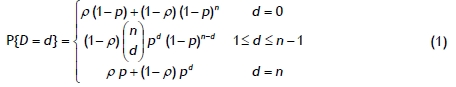
where D is the total number of nonconforming items observed within a sample. Since the probability of a sample of normal size containing more than one nonconforming item is very small in a high-yield environment, it is reasonable to define a sample as nonconforming if it contains one or more nonconforming items, and define a sample as conforming if it contains no nonconforming items. As a result, the probability of taking a nonconforming sample is given by

Let GCCC denote the cumulative count of conforming samples until the first nonconforming sample is encountered. As each sampling is independent, the GCCC statistic can be modelled by the geometric distribution with parameter p_n , and plotted over time on the chart with the upper control limit (UCL) and the lower control limit (LCL). Here we focus only on a low-sided chart, since the increase in fraction nonconforming is usually of greater concern in practice [9]. Let the acceptable rate of false alarm be denoted by α ; the LCL of the GCCC chart can then be easily obtained by

where [y ] stands for the largest integer no greater than ^y. The true false alarm rate ^α obtained from the rounded control limit may not be exactly equal to α , but is extremely close to α when p₀ is very small.

Traditionally, GCCC charts operate with fixed sampling interval (FSI) h₀ throughout the process. The VSI GCCC chart is a modification of the GCCC chart [14].

When implementing the VSI GCCC chart, a finite number of sampling interval lengths

h1,h2,...,hm (h ₁> h₂> ... > h_m ) are used, and the region above the LCL is divided by interval limits k_1;k₂,... ,km-1 (k 1 > k2 > ... > km-1 > LCL) into m sub-regions: I₁ = (k₁,∞),

Ij = (k_j,k_j-1] for j = 2,3,... m -1, and /_m= (LCL,k_m-1], corresponding to the above m

sampling intervals. The sampling interval for the subsequent inspection until the next nonconforming sample is detected depends on the current GCCC value:

In order to keep the complexity of the VSI scheme to a reasonable level, only two variable sampling intervals are used here, and thus the VSI GCCC chart divides the chart into the safety, warning, and action regions according to the warning limit (WL ) and LCL. The safety region is given by (WL,∞), the warning region is denoted by (LCL, WL ], and the action region is given by (0, LCL], where WL is also called the first interval limit (k₁).

2.2 Example

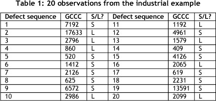
An industrial example modified from Chang & Gan [16] is presented below to illustrate the charting-and-decision procedure of VSI GCCC charts.

Consider a wire bonding process in an integrated circuit assembly that provides an electrical connection between a semiconductor die and the external leads. The machine used for wire bonding is a highly advanced machine with a closed loop control system that is able to detect and rectify any deviation generated during the wire bonding process. In such a manufacturing environment, the process yield is very high, and the percentage of nonconforming items is usually at the level of 10 ppm. For most of the time, the process remains in-control, but occasionally the non-conformance percentage shifts from the original level.

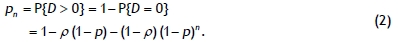
The GCCC chart with VSI scheme is employed to monitor the high-yield process. The sampling inspection of products is carried out in groups instead of sequentially, due to economy of production. With economy of scale in inspection, 50 items are sampled every time (n =50) to monitor the GCCC values. To maintain the false alarm rate at 10 for 1,000 samples on average, the acceptable false alarm rate (α ) is set at 1 per cent. The other design parameters are as follows:

ρ = 0.5, LCL=39, k₁ =2757, h₁ =1.9(min.), h₂=0.1(min.)

Table 1 lists 20 observations when the process is in-control. The results are depicted in Figure 1, where the dotted and solid straight lines are the estimated interval limit WL and LCL respectively. As shown in Figure 1, if the previous GCCC point falls into the safety region, the long interval h ₁ (loosened control mode) will be used for the subsequent inspection until the next nonconforming sample is found; otherwise the short interval h₂ (tightened control mode) will be used. Finally, if the previous sample point falls into the action region, then the process will be considered out-of-control.

 

 

 

 

3. ECONOMIC DESIGN MODEL

The model that describes the operation of the VSI GCCC chart is an extension of the model presented in Chen & Chen [13] for the VSI CCC chart. It assumes that the production process can be represented as a series of stochastically identical cycles, as follows:

1. The process starts in the in-control state with p = p₀, but after a random time of in-control operation, it will be disturbed by a single assignable cause that leads to an increase in the fraction nonconforming of a process to p = p₁.

2. Once the increase in the fraction nonconforming has occurred, the process remains out-of-control until the assignable cause is eliminated.

3. The inter-arrival time of the assignable cause disturbing the process is assumed to follow an exponential distribution with a mean of 1/λ hours.

4. To detect the increase in the fraction nonconforming, a sample is inspected at each sampling time; the number of inspected samples until a nonconforming sample occurs (i.e. the value of GCCC) is recorded and plotted on the chart in sequence.

5. Only two variable sampling intervals are used. If GCCC>LCL, the length of sampling intervals will alternate between h ₁ and h ₂ according to the position of the last GCCC point on the chart. To give additional protection against problems that arise during start-up, the initial sampling interval is set to be the short interval h ₂ to tighten the control.

6. The process will be stopped if GCCC < LCL, and a search will start to find the assignable cause and adjust the process.

7. The production cycle length is defined as the time from the beginning of the production, or after an adjustment, to the detection and elimination of an assignable cause (see Figure 2). It is usually assumed that the production cycle follows a renewal reward process.

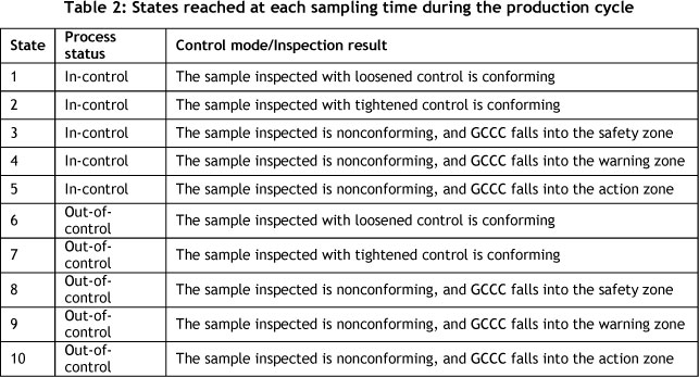
The model of Chen & Chen [13] employs a Markov chain that describes the state at each sampling time according to the actual status of the process (in-control or out-of-control under some assignable cause), the control mode (loosened or tightened control), and the inspection result (conforming or nonconforming sample). Using the above, the Markov chain has 10 states (as listed in Table 2), where states 1-9 are transient states and state 10 is the absorbing state. Note that when state 5 is reached, the signal produced by the chart is a false alarm. If the sample inspected is nonconforming and the GCCC falls into the action region when the process status is out-of-control, then the signal is a true alarm and the absorbing state, state 10, is reached.

The transition probability matrix corresponding to these 10 states is given by

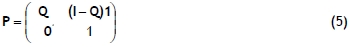
where I is the 9 χ 9 identity matrix and 1 is a 9 χ 1 column vector of ones. The rows and columns of the sub-matrix Q correspond to the in-control transition probabilities, which are given by

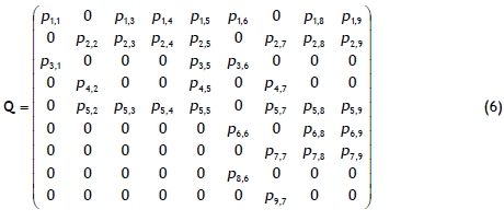
The exact expressions for the elements in matrix (6) are given in Appendix A. Note that, as shown in Appendix A, all transition probabilities in the fifth line of (6) are equal to the respective transition probabilities in the second line of (6) - that is, the transition probabilities corresponding to state 5 are equal to the ones corresponding to state 2. This is because after a false alarm, the process continues its in-control operation; and so the probability of a transition to any of the states equals to the second line as though no alarm had been issued.

In addition to equation (5), the last column in P corresponds to probabilities of moving from an in-control state to the out-of-control state, which can be obtained by subtraction since the sum of the elements in the rows of the transition probability matrix must be one.

The economic design of VSI GCCC charts is implemented by specifying a cost function and searching for the optimal design parameters to minimise the cost function over a production cycle. The production cycle shown in Figure 2 can be divided into four time intervals: an in-control period, an out-of-control period, a searching period due to a false alarm, and the time period for identifying and correcting the assignable cause. Individual periods are illustrated below before they are grouped together.

(T1) Expected length of in-control period is 1/λ .

(T2) Expected length of out-of-control period represents the average time needed for the control chart to produce a signal after the increase in the fraction nonconforming. This average time, the adjusted average time to signal (AATS ), is the most widely-used performance measure for assessing the statistical efficiency of VSI charts, and can be expressed as follows:

where ATC stands for the average time from when the cycle starts to the time the chart signals after the process change. Since the inter-arrival time of the assignable cause disturbing the process is assumed to follow an exponential distribution, the memoryless property of the exponential distribution allows the computation of ATC using the Markov chain approach, as follows:

where r' = (r1,r2,r3,r4,r5,r6,r7,r8,r9) represents the vector of starting probability; r' (I -Q)^-1 represents the mean number of transitions in each transient state before the true alarm signals; and t = (h₁,h₂,h₁,h₂,h₂,h₁,h₂,h1,h2) stands for the vector of the sampling time intervals corresponding to the nine transient states for the next sampling.

(T3) Expected length of searching period due to false alarm.

Let t₀ be the average amount of time wasted searching for the assignable cause when the process is in-control, and E(FA) be the expected number of false alarms per cycle given by

where f = (0,0,0,0,1,0,0,0,0)'. Then this expected length of searching period due to false alarm is given by t₀E(FA).

(T4) The time to identify and correct the assignable cause following an action signal is a constant t₁.

By grouping these four time intervals together, the expected length of a production cycle can be represented by

In addition, the expected net profit from a production cycle is given by

where V₀ = the hourly profit earned when the process is operating in in-control state; V₁ = the hourly profit earned when the process is operating in out-of-control state; C₀ = the average search cost if the given signal is false; C₁ = the average cost to discover the assignable cause and adjust the process to in-control state; and s = the cost for each inspected item. E(N) in (11) is the average number of inspected items during a production cycle that can be given by

where η is a column vector of sample sizes. Finally, according to the renewal reward process assumption, the expected loss per unit time E(L) is given by

 

4. OPTIMISATION PROBLEM AND SOLUTION PROCEDURE

In this study it is assumed that the process parameters (t₀,t₁,λ,p₀,p₁,ρ) and the cost parameters (s,C₀,C₁,V₀,V₁) associated with the cost function E(L) are given (or previously estimated). Then the economic design (ED) of VSI GCCC charts is to derive the design parameters (n ,WL, LCL, h₁, h₂) that minimise

E (L)

subject to

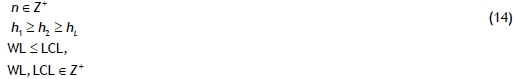
where h_L stands for the minimum time period between the samples for generating the required sample size. This minimisation problem can be regarded as a decision problem with mixed continuous-discrete decision variables and a discontinuous and non-convex solution space. It may be inefficient and time-consuming to apply typical non-linear programming techniques to a search for the optimal solution. In recent years, genetic algorithms (GAs) that were developed from an analogy with natural selection and population genetics in biological systems have been used or modified to solve the design optimisation problem of quality control charts (e.g. Aparisi & García-Díaz [17], He et al. [18], and Chen [19]). As GAs have less chance of converging to local optima in a multimodal space than do the typical techniques [17-19], we also use them to solve the optimisation problem of control charts. The solution procedure of applying the modified GAs to problem (14) is described as follows.

1. Prescribe the space of solutions (n , WL, LCL , h₁, h₂) to the design of the VSI GCCC chart. Solutions imposed by those constraints in (14) are regarded as a candidate solution.

2. Randomly generate an initial population of candidate solutions, each represented as a numerical string. The selection of population size is important for the behaviour of procedure. Small populations will run the risk of not adequately covering the search space, whereas very large populations will involve unnecessary consumption of computational time.

3. Assign each candidate solution a fitness value, which is determined by (14).

4. Select strings from the old population randomly but biased by their fitness according to the smaller-the-better rule.

5. Recombine these strings using the crossover and mutation operators. Crossover is made in the hope that new strings will have good parts of old strings and that they may be better. However, it is good to leave some part of the population to survive to the next generation. Mutation is made to prevent the search from falling into local extremes, but deviation from the random search should not occur very often.

6. Produce a new generation of numerical strings that are fitter than the previous ones.

The termination condition is achieved when the number of generations is large enough or when a satisfied fitness value is obtained.

 

5. NUMERICAL ILLUSTRATIONS AND COMPARISONS

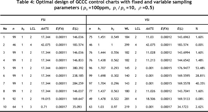
Table 3 lists diverse examples whose parameters (s,C₀,C₁,V₀,V1,t0,t1,λ) are modified from Costa [20] with a different parameter at a time. The other parameters are set as follows:

 

 

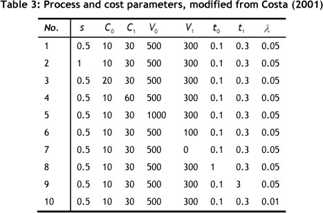
P0=100ppm; P1 /p0=10; ρ =0.5.

The economic design for the GCCC chart with FSI and VSI schemes was carried out by substituting the values of the aforementioned parameters into problem (14) and solving it by a GA optimisation package (EVOLVER 4.0.2). The following settings of control parameters for the package manipulation have been used: population size (PS)=75, crossover probability (CP)=0.1, mutation rate (MR)=0.05, and number of generations (GN) =20,000. The procedure to look for the above setting is given in Appendix B.

The 10 examples in Table 4 illustrate the savings obtained with the use of the VSI scheme for the design parameters of GCCC charts. For example, the expected unit cost E(L) in the first example reaches $146.0360 when using the FSI scheme. However, when using the VSI scheme, E(L) =$143.6963, which achieves the percentage of saving (%) in E(L) of:

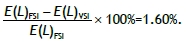
Several findings from Table 4 can be summarised:

1. It appears that the VSI control procedure requires a smaller sample size in comparison with the FSI control procedure; and in most cases the VSI control scheme outperforms the FSI one. There are enormous differences in cost saving.

2. When the cost for each inspected item s is large, or when the time spent on investigating the true alarm t₁ increases, the expected unit cost E(L) for both control procedures is the same. In such cases, the FSI control procedure is recommended, since the effort required to administer the VSI control procedure may be greater than that for the FSI one.

3. When the expected in-control time 1/λ is large, the expected unit cost E(L) becomes small, but the cost saving achieved by the VSI scheme increases only slightly.

4. An extremely large difference in profit earned per unit time between the in-control and out-of-control states (V₀ - V₁) would cause a wider difference between the long and short sampling intervals (Δ_h = h₁ - h₂), a larger sample size, a lower warning limit, and a higher cost saving achieved by the VSI scheme.

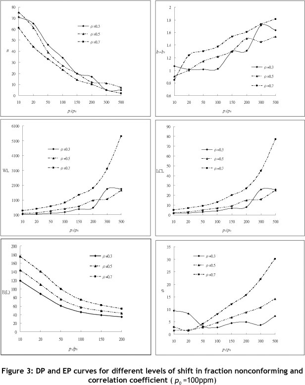
To explore further the effect of nonconforming rate p₀, process deterioration p₁ /p₀, and correlation coefficient within sample ρ on the design parameters (DP) and economic performance (EP) of the VSI GCCC chart, we first fix p₀=100ppm, and change the shift of fraction nonconforming from the original level p₁ / p₀ as well as the correlation coefficient within sample ρ. Both DP and EP curves for different levels of shift in fraction nonconforming and different correlation coefficients are shown in Figure 3, which reveals the following:

1. When p₁ /p₀ increase, both the sample size n and expected loss per unit time E(L) decrease, but the warning limit WL , the lower control limit LCL , the difference between the long and short sampling intervals Δh, and the cost saving achieved by the VSI scheme increase.

2. The cost saving achieved by the VSI scheme increases as ρ₁/ ρ₀ increases. However, it becomes insignificant when ρ is small.

Then we fix the shift of fraction nonconforming from the original level p₁ /p₀ =10, and change the values of p₀ and ρ . Both DP and EP curves for different levels of fraction nonconforming and correlation coefficient are shown in Figure 4, which reveals the following:

1. The optimal DP of the VSI chart is sensitive to the change of ρ₀ and ρ when ρ₀ is small. However, the sensitivity decreases as ρ₀ increases.

2. The cost saving achieved by the VSI scheme increases as ρ₀ increases or when ρ is small.

 

6. CONCLUSION

An economic design model, using a Markov chain, has been developed to measure the effectiveness of VSI GCCC charts from an economic point of view. The use of the model and of genetic algorithms allows the optimisation of the expected unit cost associated with the operation of VSI GCCC charts. According to the expected unit cost obtained by the newly developed models, comparisons of the VSI GCCC chart against the traditional GCCC chart with the FSI scheme are made. The numerical comparisons show that, unless the cost for each inspected item is large or the time taken to investigate the true alarm is long, using the VSI scheme in place of the FSI scheme can result in cost savings. The amount of cost savings varies depending on the process and cost parameters. When the difference in profit earned per unit time between the in-control and out-of-control states, the original level of fraction nonconforming, or the shift of fraction nonconforming from the original level is large, the amount of cost savings is more substantial.

For most of the parameter combinations considered here, the short sampling interval used in the VSI scheme is smaller than that used in the FSI scheme; meanwhile, the long sampling interval used in the VSI scheme is larger than that used in the FSI scheme. In addition, the sample size in the VSI scheme should be smaller than that in the FSI scheme. As for the lower control limit used in the VSI scheme, it is the same as that in the FSI scheme. However, the VSI should be larger than the FSI if the shift of fraction nonconforming from the original level is large, particularly when there is a large correlation coefficient within the sample.

 

REFERENCES

[1] Duncan, A.J. 1956. The economic design of X charts used to maintain current control of a process. Journal of American Statistical Association, 51, pp 228-242.         [ Links ]

[2] Montgomery, D.C. 1980. The economic design of control charts: a review and literature survey. Journal of Quality Technology, 12, pp 75-87.         [ Links ]

[3] Ho, C. & Case, K.E. 1994. Economic design of control charts: A literature review for 1981-1991. Journal of Quality Technology, 26, pp 39-53.         [ Links ]

[4] Calvin, T.W. 1983. Quality control techniques for zero-defects. IEEE Transactions on Components, Hybrids, and Manufacturing Technology, 6, pp 323-328.         [ Links ]

[5] Goh, T.N. 1987. A control chart for very high yield processes. Quality Assurance, 13, pp 18-22.         [ Links ]

[6] Xie, M. & Goh, T.N. 1992. Some procedures for decision making in controlling high yield processes. Quality and Reliability Engineering International, 8, pp 355-360.         [ Links ]

[7] Xie, M., Goh, T.N. & Xie, W. 1997. A study of economic design of control charts for cumulative count of conforming items. Communications in Statistics - Simulation and Computation, 26, pp 1009-1027.         [ Links ]

[8] Xie, M., Tang, X.Y. & Goh, T.N. 2001. On economic design of cumulative count of conforming chart. International Journal of Production Economics, 72, pp 89-97.         [ Links ]

[9] Zhang, C.W., Xie, M. & Goh, T.N. 2008. Economic design of cumulative count of conforming charts under inspection by samples. International Journal of Production Economics, 111, pp 93104.         [ Links ]

[10] Liu, J.Y., Xie, M., Goh, T.N., Liu, Q.H. & Yang, Z.H. 2006. Cumulative count of conforming chart with variable sampling intervals. International Journal of Production Economics, 101, pp 286-297.         [ Links ]

[11] Chen, Y.K., Chen, C.Y. & Chiou, K.C. 2011. Cumulative conformance count chart with variable sampling intervals and control limits. Applied Stochastic Models in Business and Industry, 27(4), pp 410-420.         [ Links ]

[12] Tagaras, G. 1998. A survey of recent developments in the design of adaptive control charts. Journal of Quality Technology, 30, pp 212-231.         [ Links ]

[13] Chen, Y.K. & Chen, C.Y. 2012. Economic design of cumulative conformance count of charts with variable sampling intervals. Arabian Journal for Science and Engineering, 37, pp 2079-2088.         [ Links ]

[14] Chen, Y.K. 2013. Variable sampling interval CCC charts for high-yield processes with correlated samples. Computers & Industrial Engineering, 64, pp 302-308.         [ Links ]

[15] Madsen, R.W. 1993. Generalized binomial distribution. Communications in Statistics - Theory and Methods, 22, pp 3065-3086.         [ Links ]

[16] Chang, T.C. & Gan, F.F. 2001. Cumulative sum charts for high yield process. Statistica Sinica, 11, pp 791-805.         [ Links ]

[17] Aparisi, F. & García-Díaz, J.C. 2004. Optimization of univariate and multivariate exponentially weighted moving-average control charts using genetic algorithms. Computers & Operations Research, 31, pp 1437-1454.         [ Links ]

[18] He, D., Grigoryan, A. & Sigh, M. 2002. Design of double and triple-sampling X control charts using genetic algorithms. International Journal of Production Research, 40, pp 1387-1404.         [ Links ]

[19] Chen, Y.K. 2004. Economic design of X control charts for non-normal data using variable sampling policy. International Journal of Production Economics, 92(1), pp 61-74.         [ Links ]

[20] Costa, A.F.B. & Rahim, M.A. 2001. Economic design of X charts with variable parameters: the Markov chain approach. Journal of Applied Statistics, 28(7), pp 875-885.         [ Links ]

 

 

* Corresponding author

 

 

APPENDIX A. DERIVATION OF TRANSITION PROBABILITIES IN Q

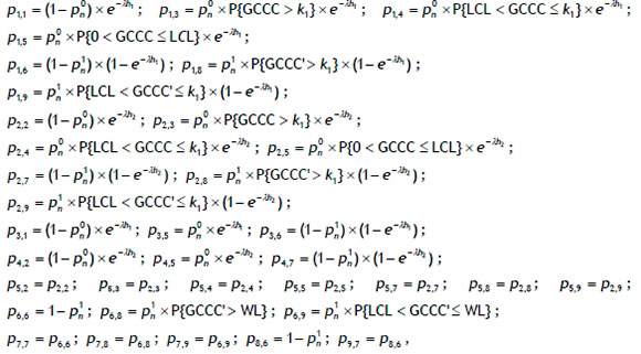
where p°_n and p¹_n denote the probability that a sample is nonconforming when the process is in-control and out-of-control, respectively; GCCC' represents a statistic that has a geometric distribution with parameter p_n¹ .

 

APPENDIX B. OPTIMAL OPERATIVE CONDITION IN GAS

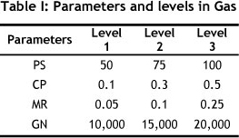
The quality of the solution generated by the GAs usually depends on the setting of their control parameters: population size (PS), crossover probability (CP), mutation rate (MR), and number of generations (GN). To find the optimal setting for these parameters, an orthogonal array experiment was developed. In the orthogonal array experiment, three levels of each parameter were planned, as shown in Table I.

 

 

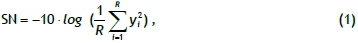
The L9 orthogonal array was employed to assign the four control parameters. In the experiment using the L9 orthogonal array, there are nine assays in total (different combinations of the four parameters). For each assay, three replicates of optimal E(L) values from the GAs, denoted by y₁, y₂, and y₃, were recorded in Table II. Because the characteristic of the objective value is smaller-the-better, the appropriate signal-to-noise ratio (SN) for evaluating the experiment results (Taguchi, 1987) is

 

 

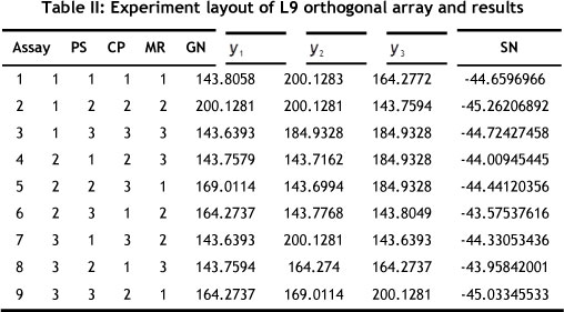
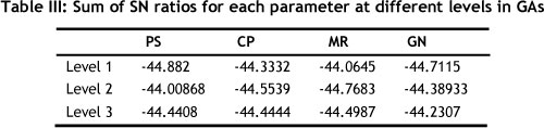
where R is the total number of replicates per assay. The values of SN ratio for each assay are also listed in Table II. Note that the SN ratio is a larger-the-better index. Accordingly, the sum of SN ratio for each parameter at different levels can be obtained as shown in Table III. According to the information in Table III, the optimal combination of the four parameters in the GA are selected by PS=75, CP=0.1, MR=0.05, and GN=20,000.