GENERAL ARTICLES

 

Statistical analysis of Caterpillar 793D haul truck engine data and through-life diagnostic information using the proportional hazards model

 

 

W.A. Carstens^{I, *}, ¹; P.J. Vlok^II

^IDepartment of Industrial Engineering Stellenbosch University, South Africa. wiehahncarstens@gmail.com
^IIDepartment of Industrial Engineering Stellenbosch University, South Africa. pjvlok@sun.ac.za

 

 

---

ABSTRACT

Physical asset management (PAM) is of increasing concern for companies in industry today. A key performance area of PAM is asset care plans (ACPs), which consist of maintenance strategies such as usage based maintenance (UBM) and condition based maintenance (CBM). Data obtained from the South African mining industry was modelled using a CBM prognostic model called the proportional hazards model (PHM). Results indicated that the developed model produced estimates that were reasonable representations of reality. These findings provide an exciting basis for the development of future Weibull PHMs that could result in huge maintenance cost savings and reduced failure occurrences.

---

OPSOMMING

Fisiese batebestuur (FBB) is besig om 'n groter bekommernis te word vir maatskappye in die bedryf vandag. 'n Sleutel fokusarea van FBB is bateversorgingsplanne wat bestaan uit strategieë soos gebruikgebaseerde onderhoud en toestandgebaseerde onderhoud (TGO). Data verkry uit die Suid-Afrikaanse mynbedryf is gemodelleer met behulp van 'n TGO prognostiese model genoem die proporsionele gevaarkoersmodel (PGM). Resultate het daarop gedui dat die model beramings verkry wat akkurate voorstellings van die werklikheid is. Hierdie bevindinge bied 'n opwindende basis vir die ontwikkeling van toekomstige Weibull proporsionele gevaarkoersmodelle wat kan lei tot groot onderhoudkostebesparings en verminderde falings.

---

 

 

1. INTRODUCTION

Only recently has industry begun to realise how ineffectively maintenance activities are performed. Heng [1] states that up to half of the maintenance performed is ineffective. This is a major concern, because maintenance is directly related to asset reliability and availability. For this reason, industry is experiencing an increased interest in physical asset management (PAM) to improve several asset-related activities in its attempt to optimise asset use.

The definition of PAM, according to the British Standards Institute's Publicly Available Specification [2], is the systematic co-ordination of activities and practices through which an organisation optimally manages its assets, and the associated performance risks and expenditures over the assets' life cycles to achieve its organisational strategic plan. The concept of PAM has several key performance areas (KPAs) - one being asset care plans (ACPs). These plans require the implementation of maintenance strategies to improve asset reliability, availability, and performance. ACPs consist of many tactical and non-tactical maintenance strategies.

Non-tactical maintenance strategies imply that maintenance is driven by assets, since assets are operated to the point of failure. Maintenance actions are performed to repair or renew unplanned failures. 'Unplanned' means that there are no procedures in place to handle failure once it occurs. Note that unplanned failures and unexpected failures are different. All failures are unexpected, although it is possible to put the necessary contingency plans in place in an attempt to manage unexpected failures.

In contrast to non-tactical ACPs, tactical ACPs ensure that maintenance is in charge of the assets. Two examples of tactical maintenance include usage based maintenance (UBM) and condition based maintenance (CBM). UBM bases its maintenance activities on historical failure data, and does not take the condition of the item into account. Historical failure data is information about the asset's previous failures, such as the time and condition of the asset at the time of failure.

CBM bases its maintenance activities on condition monitoring (CM) information, disregarding historical failure data. CM information is extracted using diagnostic sensors placed on an asset.

A major problem in South Africa is the lack of commitment to the recording of good quality data to improve maintenance decision making. A typical example of this is the mining haul trucks at Kumba Iron Ore's flagship mine, Sishen. This iron ore mine has eight Caterpillar 793D (CAT) haul trucks, and each truck has an on-board computerised maintenance management system (CMMS) that monitors and records several conditions of the truck. The mine also has a state-of-the-art tribology centre that analyses oil samples weekly. Two types of diagnostic data are recorded: a) on-board CM measurements, and b) oil analysis results.

Each truck also has an electronic control module (ECM) that uses engine management software to monitor, protect, and control the engine using its diagnostic sensors to measure several important conditions of the truck. These sensors take the operating conditions and power requirements into account to ensure that maximum performance and efficiency are achieved. On-board measurements are made hourly, where the maximum or average for that hour is taken, depending on the condition being measured. Some of the measurements include air filter pressure (kPa), ambient air temperature (°C), turbo boost pressure (kPa), and left exhaust temperature (°C).

Oil samples are taken weekly, with the constituents determined in parts per million (ppm). Other information such as viscosity is also determined with this analysis. These elements can be used to determine, to some extent, the condition of the engine and how the engine is deteriorating. Typical constituents include Fe (iron), Cr (chrome), Pb (lead), VI (viscosity I), and V40 (viscosity 40).

Maintenance is based on the oil analysis results, and on-board recordings are rarely used for maintenance decision-making. However, for each oil constituent and property, a maximum, minimum, and gradient limit is set. Maintenance is initialised if one of the three limits is reached. Data used for maintenance decision-making therefore only consists of CM data. Even though several of these data recordings are made, historical failure data is not taken into account to assist maintenance decision-making.

For this reason, this study was undertaken to research models that take into account both CM data and historical failure data. Relevant literature was researched to gain a detailed understanding of models that can be used to incorporate both types of data. Some forms of CBM have prognostic capability; this incorporates both types of data, and is discussed in the next section.

 

2. PROGNOSTIC APPROACH

CBM bases its maintenance decisions on CM data, disregarding historical failure data. CM data is used to detect worsening conditions of equipment, and to undertake maintenance action to restore equipment to an acceptable state before failure occurs. Maintenance action is taken when the health of the asset deteriorates to a predefined failure level.

CM data is also known as explanatory variables or concomitant information, and can be categorised into either quantitative or subjective data. Quantitative data includes (but is not limited to) measurements of temperature, tribological information, vibration, pressure, oil content, and stress. Subjective data is known as indicator variables and might include whether oil was changed at each service interval, what type of oil was used, which maintenance team was used, the type of installation set-up, and which supplier was used. Note that data may be time-dependent or time-independent.

Although the recording of CM data is done rigorously (and at great expense), it is rarely analysed to enhance maintenance decision-making. With accurate data it is possible to define a failure condition accurately for a certain condition being measured. Once the asset condition reaches this failure condition, maintenance action is initiated to repair or renew the asset before failure occurs. Where only one asset condition is being measured, it is reasonably simple to define a failure condition and failure.

Complex and expensive assets, however, measure several different conditions to obtain as much information about the health of the asset as possible. When several conditions are being measured, failure definition becomes extremely complex. Each of the conditions being measured might lead to failure, and analysing one condition is not enough to prevent failure. The problem is that establishing a predefined failure condition when several conditions are being measured is complex, due to the intricacy of identifying a correlation between the conditions being measured. However, certain advances in CBM have addressed this problem.

CBM has two approaches; diagnostics and prognostics. Diagnostics takes CM data into account to determine whether a predefined failure condition is reached. If this condition is met, maintenance action is initiated. A major drawback of diagnostics is that it only uses one condition to define a failure condition. Prognostics, on the other hand, combines both CM data and historical failure data to estimate future asset conditions and to identify a certain failure condition. Prognostics is thus a suitable tool for the problem at hand.

From the literature it was found that prognostic approaches have been widely applied in the field of reliability in many different industrial applications. Most prognostic approaches are based on reliability equations. These equations are used to estimate the underlying failure behaviour of the item being studied. Once these estimates are determined, it is possible to incorporate them into decision models to determine improved maintenance intervals. The following discussion is a brief overview of reliability theory and the relevant equations.

 

3. RELIABILITY THEORY

Reliability theory is focused on estimating the probability of failure or the reliability of a certain item, based on historical failure data. Four reliability equations of interest are given below.

• Probability density function, f, which is the probability that an item that has not failed in the interval (0; x) fails in the interval (x; x + δx).
• Cumulative failure distribution or survivor function, F, which is the probability that an item fails in the interval (0; x).
• Reliability function, R, which is the probability that an item does not fail in the interval (0; x).
• Force of mortality (FOM) is the instantaneous failure rate of an item that is working correctly at time x in the interval (x; x + δx).

These functions form the basis of reliability theory, and are all related in some way; if one function is known, it is possible to derive the other three. Regression models are able to model CM data together with historical failure data. Regression models are frequently used in the literature to determine reliability functions; this is because it is possible to include explanatory variables, i.e. CM data.

Several regression models were identified and compared according to their future potential in the reliability field, their implementation intricacy, their application in the reliability field, and their flexibility. These include the proportion odds model, additive hazards model, proportional hazards model, accelerated failure time model, proportional intensity model, and extended hazard regression model. After these models were evaluated, the proportional hazards model (PHM) was found to be most suitable for the problem at hand. The PHM was found to have several successful previous applications in the reliability field and good future potential, and it was extremely flexible.

 

4. PROPORTIONAL HAZARDS MODEL

The PHM, developed by Cox [3], was initially intended for the biomedical industry. It is a product of an arbitrary and unspecified baseline FOM, h₀(x), and a functional term . Knowing how maintenance decisions for the haul trucks are currently made, the problem is that failure might occur which can be indicated by more than one condition being measured. For this reason, it is necessary to determine whether there is a correlation between more than one of the properties of the haul trucks being measured, and failure. With the PHM it is possible to include on-board recorded values in conjunction with oil analysis values, to develop a PHM model that describes the underlying failure behaviour of the haul trucks.

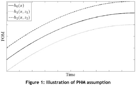
It is necessary to define the PHM assumptions before the discussion continues. These assumptions are the following:

• Variables that affect the failure times of the items are included in the model.
• For any two sets of time-independent explanatory variables, z₁ and z₂, for a single item, their associated FOM values are proportional with respect to time. Note that this assumption only holds for time-independent explanatory variables.

The first assumption states that all the environmental influences affecting the failure times of the item being studied are included in the model. For the second assumption, two sets of time-independent explanatory variables are assumed to have proportional FOM functions. These two functions, h₁(x,z₁) and h₂(x,z₂) , are also proportional to the baseline FOM h₀(x,z). Figure 1 illustrates the second assumption.

 

 

Furthermore, due to the construction of the model, explanatory variables act multiplicatively on the FOM. The functional term , can take several different forms.

A key advantage of this model is that no assumption has to be made about the baseline FOM. Consider that failure time X > 0 and a vector of m explanatory variables has been observed, i.e. . Consider also a regression coefficient of m regression coefficients, i.e. 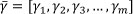. A common form of the baseline FOM found in the literature is the Weibull distribution, which is given by:

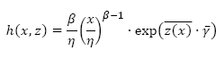
where β and η are known as the shape and scale parameters respectively. This form of the PHM is known as the Weibull PHM, and was presented by Jardine et al. [4]. Authors such as Ghasemi et al. [5], Tian & Liao [6], and Wong et al.[7] applied the Weibull PHM in the field of reliability.

4.1 Regression coefficient estimation

To determine the model parameters of the PHM, Vlok [8] indicated that the log-likelihood function should be maximised to yield the model parameters, i.e. β, η, and . The log-likelihood equation is given by:

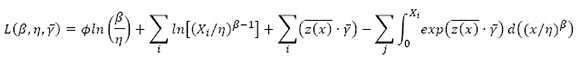
with Φ being the number of failures, i the indexing failures, and j the censored observations. (A censored observation is when maintenance is performed before an asset fails.) Failures and censored observations are collectively called 'events'. Several multivariate optimisation techniques can be used to maximise the log-likelihood function. In this study, the log-likelihood function was maximised using an algorithm developed by Carstens et al.[9]; this is a variation of a metaheuristic optimisation algorithm called the artificial bee colony algorithm.

 

5. WEIBULL PHM FIT

The main objective of model development is to determine the most appropriate explanatory variables for the best model fit. To validate the final model, seven of the eight CAT haul trucks were used to develop the final Weibull PHM model. The model was then applied to the eighth truck's data, to validate its ability to represent the failure behaviour of the eighth truck. Deciding which haul truck to use as the eighth truck was done randomly, as they all exhibit similar failure patterns.

5.1 Explanatory variable selection

Selecting explanatory variables for this study was initially done based on the experience of the engineers at the tribology centre and technicians at the maintenance workshop. They identified a total of 15 explanatory variables to be used for model development. To determine the most appropriate explanatory variables for a good Weibull PHM fit, several explanatory variable combinations were chosen and analysed to determine which variable produced the model that best fitted the data. Explanatory variable combinations were analysed and compared using goodness-of-fit (GOF) tests.

The Kolmogorov-Smirnoff (K-S) GOF test was used to determine the best explanatory variable combination. This test compares an empirical distribution with a theoretical distribution. The empirical distribution is constructed using the actual event times of the haul trucks, whereas the theoretical distribution is constructed using the explanatory variable combination and the reliability equations. These distributions are then compared to determine the accuracy of the theoretical distribution.

A test statistic D_n, is the maximum vertical distance between the two distributions, and is compared with a critical value c_nja, which is based on the number of events and the confidence interval. If an explanatory variable combination produced a test statistic less than the critical value, it can be said that there is not enough evidence to reject the null hypothesis, which states that the two distributions are equal.

The haul truck data contained 19 events, and the test was done at a confidence interval of 95%, which meant that the critical number was c_nja = 0.301. Several combinations were tested, and the best model fit produced a test statistic of 0.1731. This meant that there was not enough evidence to reject the null hypothesis because the test statistic was less than the critical value, indicating that the explanatory variable combination provided an acceptable model fit.

The explanatory variables that produced the best model fit were Fe (iron in ppm), turbo boost pressure (kPa), and left exhaust temperature (°C). These variables were used to determine the final Weibull PHM. Each variable was indicated as Fe (z₁), turbo boost pressure (z₂), and left exhaust temperature (z₃). After regression coefficient estimation was done, the final Weibull PHM model was given by:

where β = 0.833 and η = 365.542. This function represented the FOM of the haul truck data with which the decision model calculations were done. The decision models are discussed in the following section.

 

6. DECISION MODEL

Once the model parameters are determined through maximisation of the log-likelihood function, the estimates, together with the reliability equations, can be used to determine improved maintenance decision instants, using instant decision models. This section discusses two decision models: (a) residual useful life (RUL) and (b) cost optimisation. Several other models can be found in the literature, but these models were found to be the most appropriate for the specific application.

6.1 Residual life estimation

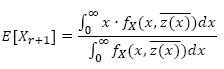
The first decision model presented is the RUL estimate that predicts the time remaining before asset failure. The expected RUL at x ≈ 0 is given by:

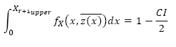
Using this equation it is possible to find the upper confidence limit by numerically solving:

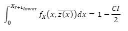
where CI is the confidence interval. The lower confidence limit can similarly be determined with:

It might seem obvious to take maintenance action when the lower RUL limit is zero. However, inspection intervals are performed discretely, and if the lower limit is close to zero at the inspection interval, it might decrease to zero between maintenance intervals, placing the item at high risk of failure before the next maintenance interval. Note that although an item is always at risk of failure, in this case the decision model cannot be used.

Perform maintenance according to the residual useful life estimates - i.e.

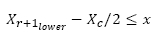
where X_r+1lower is the lower confidence limit, Xc the inspection interval, and χ the current point in time. The inspection interval X_c, is the interval at which maintenance is performed. At the Sishen mine, the haul truck's on-board measurements are made hourly. For this reason, the most convenient process parameter is time, measured in hours.

6.2 Cost optimisation model

The next model is the cost optimisation model, which attempts to minimise the long term life cycle cost of an item. The model balances two factors: (a) the cost of preventive maintenance, and (b) the cost of unexpected failure. Preventive maintenance is performed in attempt to prevent the occurrence of failure.

Let C_f indicate the cost of unexpected failure replacement and C_p the cost of preventive replacement. R_x and F_x are the reliability and survivor function respectively. Also, the time required for preventive replacement is represented by a,and the time required for failure replacement is represented by b.The cost of maintenance per unit time is then given by:

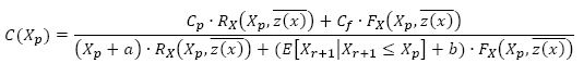
where the minimum cost is found where dC(X_p)/dx = 0, i.e. the optimal maintenance instant X_p . Perform maintenance according to the optimal point on the cost function:

x = X_p

Here x is the current point in time, and X_p is the recommended preventive replacement time. To use both decision models, a third decision model is introduced that incorporates both of these decision models.

6.3 Combined decision model logic

Two decision models were introduced: (a) RUL and (b) long term cost optimisation. To use the previous two decision model estimations fully, both decision models are combined so that maintenance is performed whenever either of the two decision models suggests that maintenance should be performed to prevent failure. To determine the effectiveness of the three decision models, each decision model was applied to the haul truck case study. The results are discussed in the following section.

 

7. MODEL VALIDATION

To test the validity of the model, it was applied to the eighth haul truck's data to estimate the truck's event times. This truck's data was handled as follows:

• Data up to a specified inspection point k x X_c, is extracted from an event's history, where k is the inspection interval number. It makes practical sense to determine estimations weekly because oil samples are taken weekly.
• At point k x X_c, an estimation is made into the future from the point of inspection, up to the point where the survivor function approaches zero, indicating zero reliability.

Because there is no data available from the point of inspection onwards, explanatory variable behaviour had to be extrapolated into the future.

7.1 Decision model estimations

The data for the eighth haul truck consisted of five events. At each inspection interval, decision model estimations were made to determine the actual event arrival times. Figure 2 illustrates the different event estimations, together with the actual event times. Each inspection point is listed under its corresponding event.

 

 

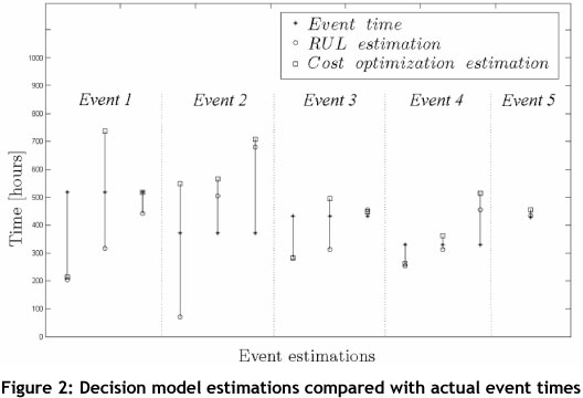
The first two event estimations were not as accurate as the last three event estimations, because the data for the first two was of lower quality than that for the third, fourth, and fifth events. From Figure 2, these event estimations can be seen to be relatively accurate, compared with the actual event arrival times.

The first two estimations of the first event were found to be inaccurate. The problem was that data obtained for this event was minimal; this meant that the model did not have enough information to predict accurately the arrival time of the first event at the first two inspections.

Another reason might be that the assumptions about future explanatory variable behaviour could be too conservative, because four of the six estimates are earlier than the actual event time. Estimations of the second event were also found to be slightly inaccurate. Further investigation indicated that several assumptions had to be made about the explanatory variables. Seeing that five of the six estimations (RUL and cost optimisation) were later than the actual failure times, assumptions regarding future explanatory variable behaviour were found to allow too high a level of risk.

However, the third estimation coincided with the failure time itself. This is because there was sufficient data with which the model could accurately predict the event arrival time. Estimates for the third event were rather conservative because three of the estimates were earlier than the actual event times. As a consequence, assumptions regarding future explanatory variable behaviour for this event proved too conservative.

If the assumptions made about the future explanatory variable behaviour proved to be too conservative, the data indicates that the haul truck is in a 'worse' state than it actually is, resulting in conservative estimations. If, however, the assumptions made about the future explanatory variable behaviour are proven to exhibit a high level of risk, the data indicates that the truck is in a 'healthier' state than it actually is, which leads to estimations with a certain level of risk.

Estimates of the fourth event indicated that the assumptions regarding future explanatory variable behaviour were also exposed to allowing too high a level of risk. Relative to the actual event times, the final three event estimates proved to be sufficiently acceptable.

This meant that it was possible to model a haul truck's failure behaviour using the Weibull PHM. The estimations indicated that the model was a relatively good representation of reality, and could be used either to replicate or to improve current maintenance decisions, i.e. ACP development.

7.2 Decision model selection

For each inspection's estimation, a percentage error value was determined. Percentage error values are calculated using the following expression:

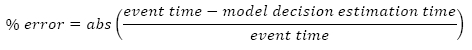
The percentage error illustrates the error of the decision model estimation based on the actual event time. This method compares the decision models in a crude but effective way.

For each decision model, an error percentage was calculated for each event. These percentages were then added to arrive at a grand total for each decision model. The first, second, and third total error percentages were 4.262, 3.943, and 4.253 respectively. Therefore the second decision model, the long term cost optimisation decision model, proved to be most successful, and should be considered for improved ACP development.

 

8. CONCLUSION

PAM is of increasing concern to industry today. A key performance indicator of PAM is ACP, which consists of several maintenance strategies. CBM is a maintenance strategy consisting of diagnostics and prognostics. Diagnostics bases its maintenance activities solely on CM data. Prognostics, however, bases its maintenance activities on CM data and historical failure data.

A prognostic model that is widely used in reliability is the PHM. Data from the mining industry was obtained, and the PHM was fitted to this data to assist in ACP development. This meant that a PHM was developed using the data obtained.

Two major benefits of the developed PHM are: a) the possibility of making relatively accurate estimations compared with the arrival times of events; and b) reduced dependence on the expertise and experience of engineers and technicians to maintain assets. From the results obtained, it is concluded that the Weibull PHM is a good representation of reality.

Although the Weibull PHM provided satisfactory results, there is still room for improvement. Estimations obtained indicate that the model was a relatively good representation of reality. The developed model can be used either to replicate or to improve current maintenance decisions. Findings from this study provide an exciting basis for the development of future Weibull PHMs that could result in huge maintenance cost savings and reduced failure occurrences.

 

REFERENCES

[1] Heng, A.S.Y. 2009. Intelligent prognostics of machinery health using suspended condition monitoring data. PhD thesis, Queensland University of Technology, Australia.         [ Links ]

[2] BSI, PAS. 2008. 55-2: Asset Management. Part 2: Guidelines for the application of PAS 55-1. British Standards Institution.         [ Links ]

[3] Cox, D. 1972.Regression models and life tables. Journal of the Royal Statistical Society Series, 1, pp. 187-220. ISSN 21.         [ Links ]

[4] Jardine, A., Anderson, P. & Mann, D. 1987. Application of the Weibull proportional hazards model to aircraft and marine engine failure data. Quality and Reliability Engineering International, 3(2), pp. 77-82.         [ Links ]

[5] Ghasemi, A., Yacout, S. & Ouali, M. 2009. Parameter estimation for condition based maintenance with proportional hazard model, International Conference on Industrial Engineering Systems and Management, IESMLinks ] Arial, Helvetica, sans-serif" size="2">.

[6] Tian, Z. & Liao, H. 2011. Condition based maintenance optimization for multicomponent systems using proportional hazards model. Reliability Engineering & System Safety 96.5:581589.         [ Links ]

[7] Wong, E., Jefferis, T. & Montgomery, N. 2010. Proportional hazards modelling of engine failures in military vehicles. Journal of Quality in Maintenance Engineering, 16(2), pp. 144-155Links ] Arial, Helvetica, sans-serif" size="2">.

[8] Vlok, P.J. 2001. Dynamic residual life estimation of industrial equipment based on failure intensity proportions. PhD thesis, Department of Industrial and Systems Engineering, University of Pretoria.         [ Links ]

[9] Carstens, W., Vlok, P.J. & Visser, T. 2011. Estimation of multivariate proportional hazards model parameters with artificial bee colony optimization. Proceedings of the 40th Conference of the Operational Research Society of South Africa (ORSSA), Elephant Hills Hotel, Victoria Falls, Zimbabwe, Operations Research Society of South Africa 2012: 51-58.         [ Links ]

 

 

* Corresponding author
1 The author was enrolled for an MSc Eng (Industrial) degree at the Department of Industrial Engineering, University of Stellenbosch.