GENERAL ARTICLES

 

The effects of incorporating vehicle acceleration explicitly into a microscopic traffic simulation model

 

 

A.P. Burger^I; M.D. Einhorn^{II, *, 2}; J.H. Van Vuuren^III

^IDepartment of Logistics Stellenbosch University, South Africa. apburger@sun.ac.za
^IIDepartment of Logistics Stellenbosch University, South Africa. einhorn@sun.ac.za
^IIIDepartment of Logistics Stellenbosch University, South Africa. vuuren@sun.ac.za

 

 

---

ABSTRACT

Explicitly incorporating individual vehicle acceleration into a traffic simulation model is not a trivial task, and typically results in a considerable increase in model complexity. For this reason, alternative implicit techniques have been introduced in the literature to compensate for the delay times associated with acceleration. In this paper, the claim is investigated that these implicit modelling techniques adequately account for the time delays due to vehicle acceleration; the modelling techniques are implemented in a simulated environment, and compared with models in which vehicle acceleration has been incorporated explicitly for a number of traffic network topologies and traffic densities. It is found that considerable discrepancies may result between the two approaches.

---

OPSOMMING

Die eksplisiete insluiting van individuele voertuigversnellings in verkeersimulasiemodelle is nie 'n maklike taak nie en veroorsaak gewoonlik 'n noemenswaardige toename in modelkompleksiteit. Om hierdie rede word alternatiewe tegnieke in die literatuur voorgestel, waarmee daar vir die vertragings wat met voertuigversnelling gepaardgaan, implisiet gekompenseer kan word. In dié artikel word die bewering dat hierdie implisiete modelleringstegnieke genoegsaam vir vertragings as gevolg van voertuigversnelling voorsiening maak ondersoek deur hierdie tegnieke in 'n gesimuleerde omgewing te implementeer en te vergelyk met modelle waarin voertuigversnelling vir verskeie verkeersnetwerktopologieë en verkeersdigthede eksplisiet geïnkorporeer is. Daar word gevind dat noemenswaardig verskillende resultate uit die twee benaderings verkry mag word.

---

 

 

1. INTRODUCTION

In simulation modelling there is usually a trade-off between model accuracy and computation time [9], with the computation time required typically increasing rapidly as model accuracy increases. This is certainly true in instances of simulation models that involve the movement of vehicles in industrial and civil engineering applications. Typically it is desirable to know how long it takes for a vehicle to complete a trip, and to determine the length of any delays it may encounter en route. One of the most common causes of a vehicle being delayed is having to stop, as well as the deceleration and acceleration on either side of the stop. Explicitly incorporating the acceleration of vehicles into a simulation model greatly increases the complexity of the model and results in longer computation times (depending on the size of the model). For this reason, measures are sometimes taken to avoid modelling vehicle acceleration explicitly. For example, Biermann [2] presents a simulation model involving a factory using automated guided vehicles (AGVs), in which it is assumed that the vehicles travel at a constant speed. This constant speed was chosen such that it compensates for the time vehicles take to reach a desired travelling speed between stops. This was done by calculating the average speed of the vehicle for the average distance before a stop, and this constant speed was used in the simulation model to determine the travel time of vehicles. Another cause of vehicle delay is traffic congestion - a phenomenon that prevents vehicles from travelling freely [20]. In another example involving the movement of forklifts in a factory, Zhang [20] describes the expected travel time of a forklift traversing a link as the sum of the vehicle movement time, the delay due to pedestrian or vehicle interruptions during travelling, either along an aisle or at an intersection, and the delay time at an end node where a forklift drops off and/or picks up stock. In this instance, the delays due to vehicle acceleration and deceleration were modelled explicitly by incorporating vehicle rates of acceleration and deceleration. A third example is the instance of modelling vehicle delays in a traffic network, which forms the basis of this paper. Vehicle acceleration forms an integral part of traffic simulation at a microscopic level as it is associated with vehicle delays, both as vehicles decelerate to join a queue and as they accelerate out of a queue [4], particularly for traffic networks that contain signalised intersections.

Due to the complex nature of modelling vehicle acceleration and deceleration, certain techniques have been introduced in the literature for incorporating the delay times associated with them effectively, without having to model the acceleration and deceleration of each vehicle explicitly. For example, Allsop [1] investigates the expressions derived by Webster [18], Miller [10], and Newell [11] for the average delay per vehicle at a signalised intersection. The work of the latter is based on a continuum model in which the individual properties of the vehicles, such as speed and position, are not considered, but rather the average and saturation flow-rates along the individual road sections adjoining an intersection. Allsop [1] presents delay expressions for various vehicle arrival and departure models. The derivation of each of the expressions relies on the aforementioned average and saturation flows of vehicles along a road section and on the timing parameters associated with the traffic signal controls at the relevant intersections. Greenshields et al. [6] attempt to account for the time delays incurred at signalised intersections due to driver reaction times and finite acceleration through the introduction of an analytically-determined constant. A similar approach is taken by Lämmer & Helbing [8].

In this paper, a comparison is made between a traffic simulation model where time delays due to vehicle acceleration are accounted for implicitly (using the above-mentioned technique proposed by Greenshields et al. [6]), and one in which vehicle acceleration is incorporated explicitly into the model. This comparison is done using the mean waiting times of vehicles present in the system and the total mean queue lengths present in the system as performance measures. The objectives are to gauge analytically the accuracy of approximating delays due to finite accelerations, and to investigate claims that it is sufficient to account for these time delays by the introduction of an analytically- determined constant, rather than incorporating the accelerations explicitly into the model. It is found that large discrepancies may result between the two approaches, depending on the size and parameters of the model. The reason for this discrepancy is that the models that incorporate acceleration implicitly cannot adequately account for the effects of congestion, which are automatically accounted for when vehicle accelerations are incorporated explicitly.

The dynamics of vehicle delays at signalised intersections are discussed in Section 2. In Section 3, a number of the differences are highlighted between vehicle delay estimations of analytic models and three commercial traffic simulation models. This is followed in Section 4 by a description of the methods followed to implement a simulation model in which vehicle accelerations are modelled explicitly and one in which they are not, but in which the delays are implicitly represented by the introduction of an analytically-determined constant. The experimental design is described in Section 5, and this is followed in Section 6 by a presentation of the results obtained and an analysis and interpretation of their significance and meaning. The paper closes with a summary in Section 7, along with suggestions for possible future work.

 

2. DELAYS AT A SIGNALISED INTERSECTION

Each signalised intersection in an urban road network represents a source of interruption of, and hence a delay in, traffic flows along the road sections converging at the intersection. This is because each traffic stream approaching a signalised intersection only receives service for a fraction of the signal's control cycle, during which vehicles belonging to that particular traffic stream may proceed through the intersection. For the remainder of the control cycle, the vehicles are required to wait for service at the intersection. However, apart from the delays that vehicles experience while waiting for service, additional delays are associated with stationary vehicles as they discharge from a queue when the traffic stream in which they find themselves starts to receive service. A brief overview is presented in this section of driver actions and subsequent vehicle movements, and of the associated delay times, when the signal turns green. In this overview we adopt the approach of an authoritative report by the South African National Transport Commission [4].

Consider Figure 1, which shows a stationary queue of n vehicles awaiting service at a signalised intersection. Upon receiving service, the vehicles begin to leave the intersection, moving towards the right of the figure. To investigate the delays incurred by vehicles as they depart from rest, the headways between consecutive vehicles are considered as they cross the stop line. The 'headway' between two vehicles is defined as the time elapsed between the crossing of the stop line by the rear of the first vehicle, and the crossing of the stop line by the rear of the vehicle following it. In the case of the first vehicle in a queue, the headway is taken as the time elapsed between the signal turning green and the rear of the vehicle crossing the stop line.

 

 

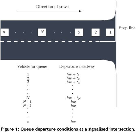
Greenshields et al. [6] observed that the headways of the first several vehicles in the queue are relatively longer than those of the vehicles that follow them. These longer headways may be explained thus: When the signal turns green, the driver of the first vehicle in the queue must observe the signal change, react to it, and then accelerate through the intersection. This results in a relatively long headway. The second vehicle in the queue follows similarly, although its driver's reaction and acceleration period partially overlaps with that of the vehicle in front of it. It also travels at a greater speed than the first vehicle as it crosses the stop line, because it has had an additional vehicle length over which to accelerate. Thus the resulting headway of the second vehicle is still comparatively long, but it is shorter than that of the first vehicle. This observation holds for the next vehicle in the queue, and so on. In this way each consecutive vehicle achieves a shorter headway than the previous one until, after a number of vehicles, N (say), the effect of driver reaction and acceleration on vehicle headways has dissipated, as shown in Figure 2.

 

 

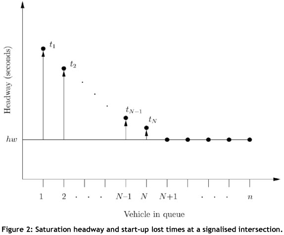
In Figure 2, the average headway achieved by vehicles after the N^th vehicle in the queue is denoted by hw. The headways of the first N vehicles, on average, exceed hw, and are expressed as hw + t_i, where t_i is the marginal headway associated with vehicle i. The value of t_i decreases as the value of i increases from 1 to N. The quantity hw is called the 'saturation headway' by the United States Transportation Research Board [16], and is used in calculating the saturation flow rate s of a road section, where s represents the number of vehicles that may pass through an intersection per hour when the saturation headway hw occurs between all pairs of successive vehicles.

The marginal headway values t₁,...,t_N in Figure 2 are also called 'start-up lost times' by the United States Transportation Research Board [16], and their sum represents the total startup lost time L of vehicles 1 to N in the queue. Each time a queue of N or more vehicles receives a green signal, the total amount of time lost is therefore the sum of hw seconds per vehicle and L.

 

3. SIMULATION MODELS VERSUS ANALYTIC MODELS

The vehicle delays described in Section 2 are considered an important performance measure for transportation systems. However, different methodologies are used to calculate these delays in simulation models and analytic models [15]. One source of analytic delay models is the Highway Capacity Manual (HCM) [17] of the Transportation Research Board, which is held in high esteem by the transportation research community and has for many years been a worldwide reference for transportation and traffic engineering scholars and practitioners, as well as the basis for several country-specific capacity manuals. Three examples of popular traffic simulation models currently in use around the world are CORSIM [3], SimTraffic [14] and VISSIM [13]. Tian et al. [15] highlight some of the differences between vehicle delay estimations in analytic models of the HCM and the three traffic simulation models. These differences are summarised below:

• The HCM reports an average control delay, which includes vehicle delays due to deceleration, queue moving time, stopped time, and acceleration. However, the HCM does not specifically take into consideration the length of an intersection approach or the speed of the approaching vehicles, which may contribute to the acceleration and deceleration portions of the control delay (e.g. higher speeds may require longer deceleration and acceleration times). In comparison, most traffic simulation models report average total delay, which is measured as the difference in travel time of a vehicle moving uninterrupted between its origin and destination, when moving at lower speeds due to congestion and traffic control implementations such as signalised intersections.
• CORSIM (Version 4.32 and earlier) and SimTraffic report total delay on a link basis. Therefore all delay due to a vehicle accelerating to its desired speed, which typically occurs on the downstream link, is not accounted for in the delay calculations. However, in CORSIM (5.0) a methodology is incorporated to take into account the acceleration so that it is consistent with the delay definition of the HCM. VISSIM, on the other hand, uses user-defined segments from which to collect delay statistics, thereby allowing for delay information to be collected; this accounts for the delay due to acceleration by correctly defining the travel time segment.
• The HCM reports delay only for the vehicles arriving during the analysis period, whereas simulation models only report delay for the vehicles departing during the analysis period. This does not result in any considerable differences when a relatively long simulation period is used (e.g. 15 minutes) in undersaturated conditions and when the total through-flow is approximately equal to all vehicle arrivals. The differences may, however, be significant in oversaturated conditions.
• Finally, a crucial difference is that simulation models automatically take into account residual queues from previous traffic signal cycles and, although the HCM provides guidelines on how to consider and account for the residual queue effect, most HCM-based analytical software packages (e.g. the Highway Capacity Software) do not compute the delay associated with residual queues.

 

4. MODELLING APPROACHES WITH AND WITHOUT VEHICLE ACCELERATION

For the case in which vehicle acceleration was incorporated into our microscopic traffic simulation model, the vehicle following philosophies proposed by Helbing et al. [7] were adopted. It was assumed that vehicles follow each other in a way such that the lower their velocity, the smaller their following distance, and vice versa. Following distances were assumed to be smallest when vehicles are stationary, in which case they are a minimum safety front-bumper-to-rear-bumper distance apart. The space occupied by a vehicle (i.e. the vehicle length plus the minimum safety front-bumper-to-rear-bumper distance) in this stationary situation is denoted by 1 /k^jam, where k^jam is the maximum traffic density (i.e. the largest number of stationary vehicles per metre on the road section). A safe following distance is assumed to be Tv_i where T is a safe time gap or reaction time maintained between consecutive vehicles, and v_i is the speed of vehicle i. The space occupied per vehicle may therefore be represented by an effective vehicle length, l^eff = 1/k^jam + Tv_i .

It was also assumed that vehicles move as fast as possible without violating the safe time gap or the speed limit, v^max. If the front vehicle travelling along a road section therefore comes within Tv^max metres of the stop line while the traffic signal is red, or if it is not able to travel through the intersection while the traffic signal is amber, the vehicle decelerates at a constant rate so as to come to a stop at the stop line. If, on the other hand, a vehicle which is not the front vehicle on the road section comes within 1 /k^jam + Tv_i metres of the vehicle in front of it, it decelerates at a constant rate such that if the vehicle in front of it were stationary, it would come to rest a distance of 1/k^jam metres behind it. If it is not travelling at the speed limit, the front vehicle along a road section accelerates until it reaches the speed limit if the traffic signal is green, and if there is sufficient space to accommodate it on the adjoining road section once it has crossed the intersection. If a vehicle is not the front vehicle along a road section, and it is not travelling at the speed limit, it accelerates at a constant rate if the distance to the vehicle in front of it is greater than 1/k^jam + Tv_i.

It was finally assumed that vehicles accelerate out of a queue from rest in such a way that vehicle i remains stationary until the distance between itself and vehicle i - 1 is at least 1/k^jam + Ta_i-1 metres, where a_i.₁ denotes the acceleration of vehicle i - 1. This corresponds to vehicle i allowing vehicle i - 1 to accelerate at the rate a_i-1 m/s² for T seconds before it starts accelerating.

For the case in which vehicle acceleration was not explicitly incorporated into our traffic simulation model, we assumed that a vehicle travels at the speed limit v^max until it reaches the stop line and the traffic signal is red (if it is the front vehicle along a road section), or until it comes within 1/k^jam metres of a stationary vehicle in front of it (if it is not the front vehicle), at which point the vehicle comes to an immediate stop. When the signal turns green, the front vehicle of the queue departs immediately at a speed of v^max, with each subsequent vehicle departing when the distance to the vehicle in front of it is at least 1/k^jam + Tv^max metres.

 

5. MODEL IMPLEMENTATION

The two microscopic traffic simulation models described above were implemented in the simulation software suite Anylogic University 6.5.0 [19]. The first step in the traffic simulation model implementation process was to build the model itself. This included the design of the road network on which vehicles travel, in terms of road section length, width, and the number of lanes, as well as points of importance along these road sections, such as entry points, stopping points, destinations, lane changes, and turning points. The length of the road sections between intersections was chosen to be 300 metres, and each road section comprised two lanes. Upon arrival at an intersection, a vehicle either turns left or right or proceeds through the intersection with equal probabilities. The next step in the model implementation was the introduction of the traffic signals that control traffic flow along the road sections at the intersections; and finally, the model was populated with vehicles.

To ensure a fair comparison of the models, all variables and characteristics of the models were kept the same. The inter-arrival times between all vehicles entering the system at each of the entry points were modelled according to a displaced exponential distribution, as suggested by Newell [12]. The probability density function of the inter-arrival times is then given by:

This displaced exponential distribution ensures a minimum inter-arrival time of T seconds between consecutive vehicles entering the system. It corresponds to a Poisson arrival process with an arrival rate of λ, interrupted immediately after each arrival by a period of T seconds, during which all arrivals that would result from the Poisson process are completely ignored.

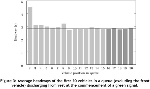
The value of T was taken as 2 seconds, while a speed limit v^max of 14 metres per second (approximately 50 kilometres per hour) was imposed. The model incorporating vehicle acceleration was run first in order to investigate the delay due to finite accelerations of the vehicles as they departed from a queue when the signal turned green. More specifically, the simulation model was run until 100 queues of at least 20 stationary vehicles had formed at a red traffic signal and departed when the signal turned green. A fixed-time signal cycle was implemented with a green time of 65 seconds, an amber time of 3 seconds, and an all-red time of 2 seconds for each conflicting traffic flow, as suggested by Lámmer & Helbing [8]. The headways between each successive pair of vehicles were recorded as the vehicles crossed the stop line of the road section, as well as the vehicles' speeds as they crossed the stop line. It was found, on average, that every vehicle after the fourteenth vehicle crossed the stopping point travelling at the speed limit, and thus the headways between the vehicles after the fifteenth vehicle were no longer affected by finite acceleration. To calculate the approximate delay due to accelerations each time a queue is discharged, the average headway between successive vehicles from vehicle fifteen to vehicle twenty was calculated. This average was then subtracted from the average headways between the first fifteen successive vehicles to cross the stop line, with the differences being summed to produce the total delay. The average headway between the vehicles after the fifteenth vehicle was found to be 2.8 seconds (which corresponds to the average headway observed between all vehicles when the same analysis was carried out for the model without vehicle accelerations). The sum by which the first fourteen observed headways exceed this average headway value was assumed to represent the delay associated with finite acceleration of the queued vehicles, and was calculated to be approximately 3 seconds.

A plot of the average headways is shown in Figure 3. The first bar represents the time elapsed between the crossing of the stop line by the first vehicle and the second vehicle, and similarly, the second bar represents the time elapsed between the crossing of the stop line by the second vehicle and the third vehicle, and so on. The reason that the headway between the signal turning green and the first vehicle crossing the stop line was not included is that it was assumed that the first vehicle reacts immediately to the green signal, resulting in a very short headway. The lighter shaded bars represent the headways of the vehicles that were still accelerating as they crossed the stop line, while the darker shaded bars represent the headways of the vehicles that crossed the stop line travelling at the speed limit. The horizontal line represents the average headways of those vehicles that crossed the stop line travelling at the speed limit.

 

 

With the delay due to acceleration calculated, it was possible to compare the two simulation models, with and without the explicit incorporation of acceleration and deceleration. For each road network topology considered, both models were run for varying values of λ (vehicle arrival rates), with each run lasting the real world equivalent of thirteen hours, and with the warm-up periods determined analytically according to the method proposed by Law [9]. The optimal green times for each value of λ were implemented for both models, with the amber time of each model being taken as three seconds. The all-red time of the model with accelerations was taken as two seconds, while that of the model with no accelerations was taken as five seconds, with the additional three seconds accounting for the delay due to acceleration, as calculated earlier. The performance measures investigated include the average waiting times of the vehicles in the system and the total average queue lengths in the system.

 

6. RESULTS AND INTERPRETATION

The results presented in this section were obtained for three different urban road network topologies: a single isolated intersection, a two-by-two grid of intersections (four intersections in total), and a three-by-three grid of intersections (nine intersections in total). For each topology, five different values of λ were considered: 0.05, 0.1, 0.15, 0.2 and 0.25.

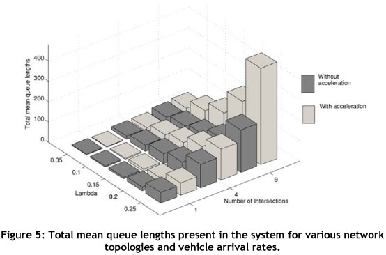
The mean waiting times of the vehicles present in the system for the different network topologies and vehicle arrival rates (λ) are shown in Figure 4, while the corresponding total mean queue lengths in the system are shown in Figure 5.

 

 

 

 

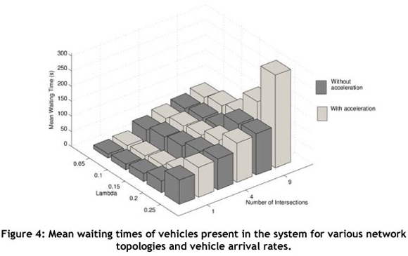
It may be seen in Figure 4 how the difference in vehicle waiting times measured by the model with vehicle acceleration and the one without vehicle acceleration grows in magnitude, both as the number of vehicles present in the system increases and as the number of intersections increases. A vehicle was considered to be queued or waiting if it was not travelling at its desired speed, which for these particular simulation models was assumed to be the speed limit. This is opposed to considering a vehicle to be waiting only if it were stationary, which would result in the vehicles in the system without vehicle accelerations to experience longer waiting times because they reach a stationary state sooner than their counterparts in the model in which accelerations are explicitly incorporated.

Einhorn [5] cites a possible explanation for these differences: that, in spite of the fact that an additional three seconds have been added to the all-red phase of the traffic signal cycle to account for delays due to finite acceleration in the simulation model that does not explicitly incorporate vehicle accelerations, the model without acceleration does not accommodate the fact that a vehicle continues to accelerate once it has passed the stop line. Attempts at artificially accounting for the time delay due to finite acceleration past the stop line (or any fixed point, for that matter) are expected to be considerably more challenging, since vehicles typically reach the speed limit at different points along the road section.

These effects are experienced by each vehicle in the system that is required to accelerate out of a queue, and are thus amplified by an increase in vehicle numbers within the system and by an increase in the number of times a vehicle becomes queued due to an increase in the number of intersections.

Another reason for the noticeable difference in vehicle waiting times measured by the two alternative models is that much larger queues are experienced in the simulation model in which vehicle accelerations are incorporated, as may be seen in Figure 5.

The longer queues experienced by vehicles in the model with acceleration are again due to an underestimation in the delay caused by finite acceleration, since the vehicles are still accelerating as they cross the stop line, and therefore travel marginally slower than vehicles that would be travelling at the speed limit (as in the simulation model without acceleration). This may result in these vehicles having to queue at the adjacent intersection, whereas if they had been travelling faster (as would be the case in the simulation model without acceleration) they may not have had to queue, as they would have arrived at the adjacent intersection while the signal was still green. This effect is again amplified by an increase in vehicle and intersection numbers, and thus the longer the queue, the more time a vehicle is likely to spend waiting in it, resulting in an increase in the mean waiting times.

 

7. CONCLUSION

Based on the above illustration of the magnitudes of the discrepancies between the results obtained by the two simulation models for mean vehicle waiting times in the system and the total mean queue lengths in the system, summarised in Figures 6 and 7 respectively, it is concluded that - while it is certainly simpler and computationally more efficient to model a real-world traffic system without incorporating vehicle acceleration explicitly - the approaches typically adopted in the literature to account for delays due to vehicle acceleration are not sufficiently accurate to represent a real world traffic system.

 

 

 

 

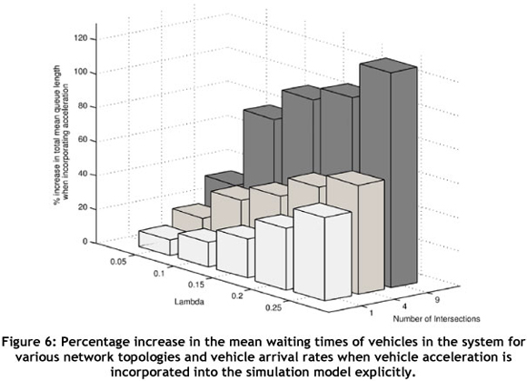
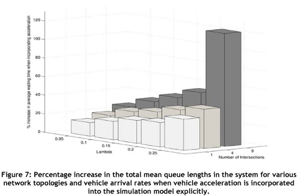
It should also be noted that these discrepancies become more pronounced as the road network topology becomes more complex, and/or as the number of vehicles in the system increases. It is therefore recommended that, depending on the size and complexity of the traffic simulation model, and the level of detail required, vehicle acceleration be incorporated explicitly into microscopic traffic simulation models, so as to improve the realism of the models and the validity of the results they produce.

We highlight two possible avenues of further investigation. The first is to investigate more detailed analytic models that are able to account for delays that result from congestion along road ways. The second is to investigate more efficient techniques of explicitly incorporating vehicle accelerations into simulation models. However, these two suggestions may soon become redundant, as commercial simulation packages are increasingly incorporating specialised traffic libraries in which vehicle accelerations are incorporated explicitly without requiring any additional computing work from the user (but still with heavier model computational burdens).

We close by noting that the work contained in this paper need not only be considered relevant for road traffic simulation models, but is applicable to any simulation model in which delay to a vehicle's travel time is important, such as in the manufacturing contexts mentioned in Section 1.

 

REFERENCES

[1] Allsop, R.E. 1972. Delay at a fixed time traffic signal: I Theoretical analysis, Transportation Science, 6(3), pp. 260 - 285.         [ Links ]

[2] Biermann, H.J. & Bekker, J.F. 2012. Multi-objective assessment of vehicles in a reconfigurable manufacturing system with discrete-event simulation, Bachelor of Industrial Engineering Fourth Year Project, Stellenbosch University, Stellenbosch.         [ Links ]

[3] COR User's Guide. 2005. CORSIM User's Guide, Version 6.0. ITT Industries, Inc., Systems Division, Prepared for Federal Highway Administration, Washington (DC).         [ Links ]

[4] Department of Transport Chief Directorate: National Roads. 1988. Guidelines for the application of traffic signal phasing and control equipment, (Unpublished) Technical Report 87, National Transport Commission, Pretoria.         [ Links ]

[5] Einhorn, M.D. 2011. An evaluation of the efficiency of self-organising versus fixed traffic signalling paradigms, M.Sc. (Operations Research) Thesis, Stellenbosch University, Stellenbosch.         [ Links ]

[6] Greenshields, B.D., Schapiro, D. & Ericksen, E.L. 1946. Traffic performance at urban street intersections, (Unpublished) Technical Report 1, Bureau of Highway Traffic, Yale University, New Haven (CA).         [ Links ]

[7] Helbing, D., Lammer, S. & Lebacque, J.P. 2005. Self-organized control of irregular or perturbed network traffic, Advances in Computational Management Science, 7(4), pp. 239 - 274.         [ Links ]

[8] Lammer, S. & Helbing, D. 2008. Self-control of traffic lights and vehicle flows in urban road networks, Journal of Statistical Mechanics: Theory and Experiment, 2008, p. P04019.         [ Links ]

[9] Law, A.M. 2007. Simulation modeling and analysis, 4^th Edition, McGraw-Hill, Boston (MA).         [ Links ]

[10] Miller, A.J. 1963. Settings for fixed-cycle traffic signals, Operations Research Quarterly, 14(4), pp. 373 - 386.         [ Links ]

[11] Newell, G.F. 1956. Statistical analysis of the flow of highway traffic through a signalized intersection, Quarterly of Applied Mathematics, 13(4), pp. 353 - 369.         [ Links ]

[12] Newell, G.F. 1965. Statistical analysis of the flow of highway traffic through a signalized intersection, SIAM Review, 7(2), pp. 223 - 239.         [ Links ]

[13] Planung Transport Verkehr AG. 2011. Vissim 5.40-01 user manual, Karlsruhe.         [ Links ]

[14] SimTraffic, 2003. SimTraffic, 6,Traffic Simulation Software - User Guide, Trafficware Corporation. Albany, 2003.         [ Links ]

[15] Tian, Z.Z., Urbanik II, T., Engelbrecht, R. & Balke, K. 2002. Variations in capacity and delay estimates from microscopic traffic simulation models. Transportation Research Record: Journal of the Transportation Research Board, 1802.1 pp. 23 - 31.         [ Links ]

[16] Transportation Research Board. 1994. Traffic highway capacity manual, (Unpublished) Technical Report 209, National Research Council, Washington (DC).         [ Links ]

[17] Transportation Research Board. 2000. Highway capacity manual, National Research Council, Washington (DC).         [ Links ]

[18] Webster, F.V. 1958. Traffic signal settings, (Unpublished) Technical Report 39, Her Majesty's Stationery Office, London.         [ Links ]

[19] XJ Technologies. 2010. Anylogic University 6.5.0. [Online], Available from: http://www.xjtek.com/.         [ Links ]

[20] Zhang, M., Batta, R. & Nagi,R. 2009. Modeling of workflow congestion and optimisation of flow routing in a manufacturing/warehouse facility, Management Science, 55(2), pp. 267-280.         [ Links ]

 

* Corresponding author.
2 The author is enrolled for a PhD (Operations Research) degree in the Department of Logistics at Stellenbosch University.