GENERAL ARTICLES

 

A study of the median run length (MRL) performance of the EWMA t chart for the mean

 

 

W.S. Chin^{I, 1} ; M.B.C. Khoo^{II, *}

^ISchool of Mathematical Sciences Universiti Sains Malaysia, Malaysia. chinwensim87@yahoo.com
^IISchool of Mathematical Sciences Universiti Sains Malaysia, Malaysia. mkbc@usm.my

 

 

---

ABSTRACT

The exponentially weighted moving average (EWMA) X chart is effective in detecting small shifts. However, the EWMA X chart is not robust enough to prevent errors in estimating the process standard deviation or a changing standard deviation. To overcome this problem, Zhang et al. suggested the EWMA t chart in 2009. The existing optimal design of the EWMA t chart is based on the average run length (ARL) criterion. This paper proposes that the optimal design of the EWMA t chart be based on the median run length (MRL). The MRL performances of the optimal EWMA X and optimal EWMA t charts are compared.

---

OPSOMMING

Die eksponensiaalgeweegde bewegende gemiddelde (EWMA) X -kaart is geskik om klein verskuiwings te bespeur. Die EWMA X -kaart is egter nie robuust genoeg om foute in die beraming van die proses standaardafwyking of 'n veranderende standaardafwyking te voorkom nie. Om die probleem te oorkom het Zhang et al. in 2009 die EWMA t-kaart voorgestel. Die bestaande, optimale ontwerp van die EWMA t-kaart is gebaseer op die gemiddelde lopielengte kriterium. Dié artikel stel voor dat die optimale ontwerp van die EWMA t-kaart eerder op die mediaanlopielengte gebaseer word. Die resultate van die gebruik van die mediaanlopielengte met die EWMA X - en die optimale EWMA t-kaarte word vergelyk.

---

 

 

1. INTRODUCTION

The EWMA control chart was introduced by Roberts [1]. Since then numerous extensions on EWMA charts have been made. Among the more recent extensions on EWMA charts are those by Su et al. [2], Graham et al. [3], Castagliola et al. [4], Tsai & Yen [5], Celano et al. [6], Yang et al. [7], Lee & Apley [8], Perry & Pignatiello [9], Lin & Chou [10], Pascual [11], Ozsan et al. [12], Simoes et al. [13], Epprecht et al. [14], Khoo et al. [15], Li et al. [16], Spliid [17], Capizzi & Masarotto [18], and Thaga & Yadavalli [19]. The EWMA X chart is excellent in detecting small persistent changes in the mean.

In the application of the EWMA chart, the process standard deviation is usually assumed to be well estimated, and does not change. Unfortunately this is not always the case in practice [20]. Therefore Zhang et al. [20] proposed the EWMA t chart to overcome this problem, by showing that the EWMA t chart is more robust than the EWMA X chart in preventing estimation errors or changes in the process standard deviation. In addition, it was shown that the EWMA t chart always has a lower size of the Type II error than the EWMA X chart for mean shifts αε[0, 0.5] when the charts are optimally designed for a quick detection of moderate and large shifts (see Figure 7 in Zhang et al. [20]). However, when the two charts are optimally designed for a quick detection of small shifts, the EWMA X chart has a slightly lower size of the Type II error than the EWMA t chart, but the difference is very small - for mean shifts αε[0, 0.5] (again, see Figure 7 in [20]).

In most situations, the average run length (ARL) or the median run length (MRL) is used to measure a chart's performance. The ARL and MRL are defined as the average and median number of sample points that are plotted on a chart before an out-of-control signal is issued. The ARL is more commonly used than the MRL in measuring a chart's performance. This is due to the relative difficulty in computing the run length distribution. Furthermore, the run length distribution is nearly geometric; hence the run length distribution can be characterised by its average, i.e. the ARL [21, 22].

Interpretations based on ARL alone can be misleading, as the in-control run length distribution of a control chart is highly skewed. The interpretations become more difficult as the shape of the run length distribution changes according to the magnitude of the shift [21, 22]. On the other hand, when using the MRL this interpretation problem will not occur. For example, even though the in-control ARL of the Shewhart chart with ±3 standard deviations width is 370, the fact is that 60% to 70% of the run lengths will be less than 370. In fact, 50% of the run lengths will be less than 257, which is the in-control MRL. Thus in using the ARL as a performance measure, a practitioner may have an incorrect understanding that half the time, an out-of-control will be signaled by the 370^th sample when the process is in-control; although in an actual situation, an out-of-control will be given by the 370^th sample 60-70 percent of the time. In fact, the in-control MRL of 257 indicates that half the time (or 50%), an out-of-control signal is issued by the 257^th sample [23]. The MRL provides a more meaningful interpretation for the in-control and out-of-control performances of a chart, and is readily understood by quality practitioners, as it gives the probability of a signal by a certain number of samples. In contrast, the ARL only provides the average number of samples to signal, which does not provide any probabilistic measure of the time to signal. Charts that are optimally designed based on MRL were presented by Gan [21, 22] and Khoo et al. [24].

The EWMA t chart proposed by Zhang et al. [20] is optimally designed when based on the ARL alone. Thus this paper studies the MRL performance of the EWMA t chart, and also provides an optimal design procedure, based on the MRL and the computed optimal parameters of the chart. The MRL performances of the EWMA t and EWMAcharts are compared. The objective of this study is to facilitate the work of quality practitioners in selecting the optimal parameters of the EWMA t chart, whose design is based on MRL.

This paper is organised as follows: Section 2 presents the EWMA chart. The EWMA t chart is given in Section 3. In Section 4, the Markov chain approach in computing the MRLs of the EWMA t and EWMA charts is discussed. The optimal design procedure for the EWMA t and EWMA charts, based on the MRL, is described in Section 5. An illustrative example is provided in Section 6. Section 7 compares the MRL performances of the EWMA t and EWMA X charts. Conclusions are drawn in Section 8.

 

2. THE EWMACHART

Assume that samples {X_f1,X_i2,...,X_i,n} are taken at time i =1,2, where n is the sample size. It is assumed that independence exists within and between subgroups, and that 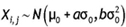, for i = 1, 2, and 1 < j < n, where µ₀ and σ₀ are the nominal mean and standard deviation respectively. The process is in-control when a = 0 and b = 1. On the other hand, the process is out-of-control when the mean has changed (a ≠ 0), or the standard deviation has changed (b ≠ 1), or both have changed.

The plotting statistic of the EWMA chart, i.e. Z_i, is defined as follows:

where λ is the smoothing constant that satisfies 0<λ<1, is the sample mean at time i with and Ζ₀=µ₀ [20]. The upper and lower control limits of the EWMA chart are

and

respectively. Here, 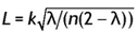, where the multiplier k is to be determined by the user, based on a desired in-control ARL (ARL₀) or in-control MRL (MRL₀).

 

3. THE EWMA t CHART

The plotting statistic Y_i for the EWMA t chart suggested by Zhang et al. [20] is defined as follows:

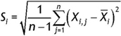
where , Here, S_i is the sample standard deviation at time i, i.e.

[20]. Note that Ti follows a t distribution with n-1 degrees of freedom, and that the t distribution is symmetrical about 0, so that E(Y_i) = E(T_i) = 0 when the process is in-control. Hence the upper and lower control limits of the EWMA t chart satisfy LCL_t = -UCL_t [20]. The UCL_t of the EWMA t chart is a function of the sample size, n, smoothing constant, λ, and MRL₀ (or ARL₀ ).

 

4. A MARKOV CHAIN APPROACH IN COMPUTING THE MRLs OF THE EWMA X AND EWMA tCHARTS

This section discusses the Markov chain approach of Brook & Evans [25] to evaluate the MRLs of the EWMA and EWMA t charts. Zhang et al. [20] also employed the Markov chain approach of Brook & Evans [25] to evaluate the ARLs of these two EWMA charts. A discrete-time Markov chain has p+1 states, where states 1, 2, p are transient while state p+1 is absorbing. Zhang et al. [20] showed that the transition probability matrix P of this discrete-time Markov chain is

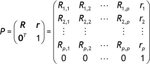
where R is the p χ p transition probability matrix for the transient states (in-control process). Then the (px1) vector r satisfies r = 1 - R1 (row probabilities must sum to 1), where 1 = (1,1,...,1)^T and 0 = (0,0,...,0)^T are both (px1) dimensional vectors. Let s^T = (s₁,s₂,...,s_p) be the (px1) initial probability vector, associated with the p transient states.

Figure 1, taken from Zhang et al. [20], shows how the interval between UCL and LCL (UCL_t and LCL_t), for the EWMA (EWMA t) chart is divided into p = 2m + 1 subintervals. For simplicity, UCL and LCL will be used to represent the limits of the two EWMA charts in this section. The width of each subinterval is 2δ, where . Note that Hj is the midpoint of the j^th subinterval, for j = -m, -1, 0, +1, ... , +m, where m denotes the subinterval number [20].

 

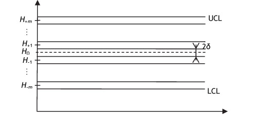
Figure 1: Interval between UCL and LCL divided into p = 2m + 1 subintervals

 

Let N denote the run length of the EWMA and the EWMA t charts. Here, N is a Discrete Phase Type random variable. The cumulative distribution function (cdf) of N for the zero state process [25] is:

where I represents the (pxp) identity matrix, s represents the (px1) initial probability vector, 1 represents the (px1) vector of all ones. The 100 γ (0 < γ < 1) percentage points of the run length distribution are defined as the value z_γ, such that [21, 22]:

By letting γ = 0.5 in equation (5), we obtain MRL = z₀₅.

The transition probability R_{i, j} of the in-control transition probability matrix R for the EWMA X chart [20] is:

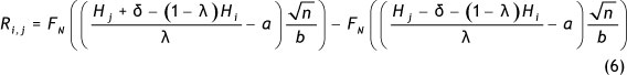
where F_N represents the cdf of the standard normal distribution. For the EWMA t chart, the transition probability, R_{i, j} of matrix R [20] is:

where F_t (·| n - 1,β) is the cdf of a non-central t-distribution with n-1 degrees of freedom and noncentrality parameter β.

The generic element s_j of the initial probability vector s for the EWMA chart [20] is:

For the EWMA t chart, the generic element s_j of vector s is

 

5. OPTIMAL DESIGNS OF THE EWMA X AND EWMA t CHARTS, BASED ON MRL

The optimal parameters of the EWMA and EWMA t charts can be computed using the Markov chain approach discussed in Section 4. A chart is optimal in detecting a shift if, among all the competing charts with the same MRL₀, it has the smallest out-of-control MRL for the said shift. The MRL is a discrete number, so it is possible that more than one optimal parameter combination exists for a particular magnitude of shift of interest. For such cases, the (λ, UCL_t) combination corresponding to the median λ of all optimal λ in the range [a, b], where 0<a<b<1, is taken as the optimal parameter combination. Note that any (λ, UCL_t) combination where λε[α, b] can be selected by the user as the optimal combination if desired.

The following steps explain how the optimal (λ, UCL_t) parameter combination of the EWMA t chart is computed:

Step 1: Specify the desired MRL₀ value, sample size, n, and mean shift a_opt, where a_opt is the magnitude of a shift for which a quick detection is needed. Here, a_opt is measured in terms of the number of standard deviation units.

Step 2: Initialize λ as 0.01.

Step 3: With the current λ value, compute the corresponding UCL_t to attain the MRL₀ specified in Step 1, when the process is in-control. Here, matrix R is obtained by setting a=0 and b=1, as UCL_t is computed based on an in-control process.

Step 4: Using the (λ, UCL_t) combination in Step 3, compute the out-of-control MRL (MRL_Qpt) for the shift a_opt whose value is set in Step 1. Here b=1 is used, as only a shift in the mean is considered.

Step 5: Repeat Steps 3 and 4 for λ ε {0.011, 0.012, 0.013, ..., 0.999, 1} so that 990 (λ, UCL_t)combinations and their corresponding MRL_aopts are obtained.

Step 6: Identify the (λ, UCL_t) combination having the smallest MRL_{a t} value. The (λ, UCL_t)combination having the smallest MRL_aopt value is the optimal parameter combination out of all the 991 (λ, UCL_t) combinations, for λ = 0.01, 0.011, 0.012, ., 1.

Note that the optimal (λ, L) parameter combination of the EWMA chart is also obtained using the above six-step procedure. However, for the EWMA chart the transition probability R_i,j in equation (6) is employed.

Statistical Analysis System (SAS) programs are written incorporating this six-step procedure to compute the optimal parameter combinations for the EWMA t and EWMA charts using the Markov chain approach. (These optimisation programs - which compute the optimal parameters for any desired input parameters (MRL₀, a_opt, and n) set by the user - can be requested from the first author.)

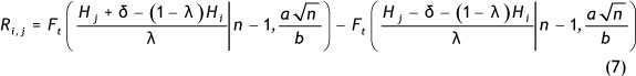
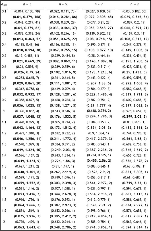
Tables 1 and 2 provide the optimal parameter combinations and the corresponding MRL_aptsfor the EWMA t and EWMA X charts, when MRL₀ ε {200, 370}, a_opt ε {0.1, 0.2, ..., 1.9, 2.0}, and n ε {3, 5, 7, 9}. The bold type entries represent the optimal parameters and MRL_aopts for the EWMA t chart. Tables 1 and 2 facilitate a quick selection of optimal parameters by a practitioner. For example, if a practitioner wishes to design an EWMA t chart that is optimal for a shift of a_opt = 0.5, when n = 5 and MRL₀ = 200, the optimal parameters that must be used are λ = 0.109 and UCL_t = 0.944, where the corresponding out-of-control MRL (MRL_a ) obtained is 10. This MRL_a value is the smallest among the out-of-control MRLs of all the EWMA t charts that are designed to have MRL₀= 200. The accuracy of the entries in Tables 1 and 2 has been verified with simulation. Here, the simulation programs for the EWMA t and EWMA X charts are written using SAS, each based on 10,000 simulated trials. (These simulation programs can be requested from the first author.) For example, to verify the accuracy of the MRL_apt value when MRL₀= 370, n = 3, and aopt = 0.8, the optimal parameters (λ = 0.032, UCL_t = 0.932) (see Table 2) are entered into the simulation program for the EWMA t chart, where the program's output shows that MRL _aopt = 17 - i.e., similar to that obtained using the SAS optimisation program. Note that the SAS optimisation program incorporates the six-step procedure discussed at the beginning of this section.

 

Table 1: Optimal (λ, L) and optimal (λ, UCL_t) combinations, and their corresponding MRL_%i , for the EWMA X and EWMA t (boldfaced entries) charts, based on MRL₀ = 200

 

 

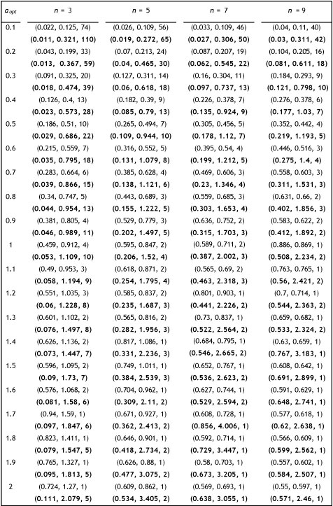
Table 2: Optimal (λ, L) and optimal (λ, UCL_t) combinations, and their corresponding MRL_%t , for the EWMA and EWMA t (boldfaced entries) charts, based on MRL₀ = 370

 

Some discussions that might be useful to the reader are presented here. The probability that a process is in-control, even though the chart indicates otherwise, is defined as the size of the Type I error. Here, fixing the value of this probability corresponds to fixing the value of the MRL₀. A higher MRL₀ value corresponds to a smaller size of the Type I error, and vice versa. On the other hand, the probability that a process is out-of-control, even though the chart does not indicate this, is the size of the Type II error. The size of the Type II error is related to the value of MRL_aopt . The value of MRL_aopt increases as the probability of the Type II error increases, and vice versa. In this section, an 'optimal' chart refers to the chart where the size of its Type I error is fixed, while the size of its Type II error for a specified shift of interest ( aopt ) is minimised. This is equivalent to the approach employed in the paper by fixing the MRL₀value and minimising the MRL_apt value.

 

6. AN ILLUSTRATIVE EXAMPLE

This example illustrates how the EWMA t chart is constructed using the data taken from a local manufacturer. To protect the manufacturer's identity, its name is not revealed. The data deal with torque measurements (in Newton cm, Ncm) for a screwing process in manufacturing a car radio. The quality characteristic of interest in the screwing process is the torque, a measure of turning force required to engage a screw to the screwing hole with an electronic screwdriver. Note that a sample of five torque measurements is taken every hour.

The Phase I data, which consist of 25 samples, each of size n = 5, are shown in Table 3. Table 3 also gives the sample mean and sample standard deviation S_i, for i = 1, 2, 25, where i denotes the sample number.

 

Table 3: Torque measurements (in Ncm) for the screwing process

 

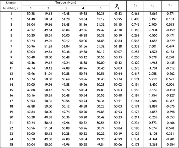
The sample grand average for the Phase I data is computed as . Then is computed for each of the 25 samples. Assume that the EWMA t chart is to be designed to be optimal for a mean shift a_opt = 0.6, where MRL₀= 200. Then the optimal parameters λ = 0.131 and UCL_t = 1.079 (see Table 1) are selected. Thus the lower control limit of the EWMA t chart is LCL_t = -1.079 because LCL_t = -UCL_t, as discussed in Section 3. The EWMA t statistics, computed using equation (3) with Y₀ = 0 and λ = 0.131, are also shown in Table 3. The EWMA t chart corresponding to the Phase I data is plotted in Figure 2. In Figure 2 no point falls beyond the limits, so the Phase I process is said to be in-control. Therefore the limits of the EWMA t chart, established in Phase I, can be used to monitor the Phase II process.

 

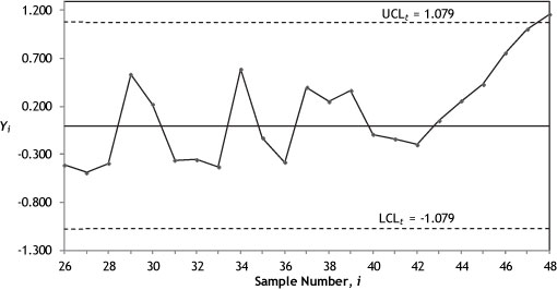
Figure 2: The EWMA t chart for the Phase I data

 

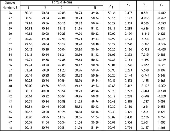
The Phase II process consists of 23 samples (samples 26-48), each of size n = 5. The sample measurements and the associated , S_i, T_i , and Y_i statistics are shown in Table 4. The EWMA t chart for the Phase II data is plotted in Figure 3. The chart detects an out-of-control point at the 48^th sample. Furthermore, the chart shows an upward trend from sample 42 onwards, indicating that the Phase II process is out-of-control. Thus an investigation should be conducted to identify the assignable cause(s).

 

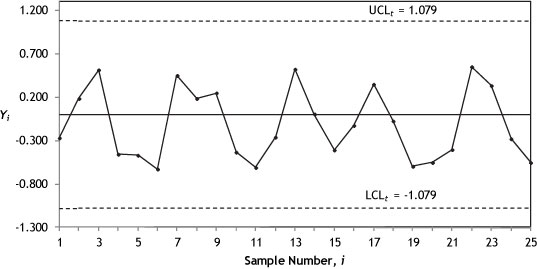
Figure 3: The EWMA t chart for the Phase II data

 

 

Table 4: 23 additional samples for the screwing process

 

7. PERFORMANCE COMPARISON

The MRL performances of the EWMA t chart and EWMA chart are compared. The optimal parameter combinations of the EWMA t and EWMA charts are selected, for MRL₀ ε {200, 370, 500}, a_opt ε {0.2, 0.7, 1.5}, and n = 5, where a_opt is the magnitude of a mean shift that needs a quick detection. Note that 0 < a < 0.5 and bε {0.90, 0.95, 1.00, 1.05, 1.10} are considered. Only the results for MRL₀ = 370 are shown in Figure 4, because the results for MRL ₀ = 200 and 500 have similar trends. The role of Figure 4 is to show the difference in the MRL values for the various b values for both EWMA charts. Figure 4 shows that the MRL curves for the EWMA X chart exhibit large differences for each of the three a_opt values.

 

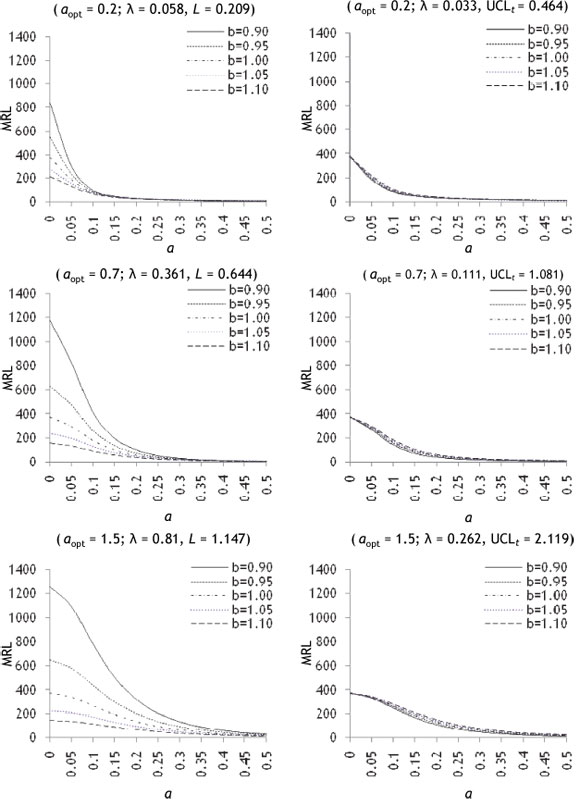
Figure 4: MRL curves for n = 5, αε[0, 0.5], be{0.9, 0.95, 1.00, 1.05, 1.10}, MRL₀ = 370, and o_opt ε {0.2, 0.7, 1.5}, for the EWMA X chart (left side) and the EWMA t chart (right side)

 

For example, when a_opt = 0.7, the MRL curves for the EWMA chart when b φ 1, display great differences from the MRL curve associated with b = 1, for a ε [0, 0.25]. Also, the MRLs, when a = 0 and b φ 1, are far from the specified target value MRL₀ = 370 (see Figure 4). The differences among the MRL curves for the EWMA chart become more pronounced when λ increases. In contrast, the MRL curves among the different values of b for the EWMA t chart in Figure 4 are hard to distinguish for each of the three values of aopt considered. The results show that the EWMA t chart is more robust in preventing changes in b than the EWMA chart.

Note that the range of the a values on the x-axis in Figure 4 is set, based on the range considered in Zhang et al. [20]. Zhang et al. [20] considered the a_opt values that did not include the range of the a values on the x-axis. Furthermore, since all the MRL curves for different b values overlap from a = 0.5 onwards (see Figure 4), it is pointless to show the curves for a > 0.5, as the differences among the curves for the various b values are not visible when a > 0.5.

This section compares the MRL performances of the EWMA t and EWMA charts. The results show that the EWMA t chart is more robust in preventing changes in b than the EWMA chart. It is also interesting to note that the optimal EWMA t chart is better than the optimal EWMA chart in detecting process mean shifts in terms of the ARL, as illustrated in Section 1, paragraph 2.

 

8. CONCLUSION

The main objective of this paper is to extend the work of Zhang et al. [20] by suggesting an optimal design of the EWMA t chart based on MRL. Its aim is not to study the chart's performance in detecting shifts, as this work has been done by Zhang et al. [20] (see Section 1, paragraph 2, line 5 onwards). As explained in Section 1, the MRL provides useful information not given by the ARL, and the former is also more readily understood by practitioners. This paper complements the work of Zhang et al. [20] who designed the EWMA t chart using the ARL. Note that the optimal designs of the EWMA chart, based on both the ARL and MRL criteria, are available in the literature. Thus the optimal design of the EWMA t chart based on MRL, as presented in this paper, should be made available to practitioners. This is because the MRL optimisation procedure of the EWMA t chart is not currently available. A comparison of the MRL curves for the EWMA and EWMA t charts shows that the latter performs better than the former against changes or estimation error in the process standard deviation.

 

REFERENCES

[1] Roberts, S.W. 1959. Control chart tests based on geometric moving averages, Technometrics, 1(3), pp 239-250.         [ Links ]

[2] Su, Y., Shu, L. & Tsui, K.L. 2011. Adaptive procedures for monitoring processes subject to linear drifts, Computational Statistics ã Data Analysis, 55(10), pp 2819-2829.         [ Links ]

[3] Graham, M.A., Chakraborti, S. & Human, S.W. 2011. A nonparametric exponentially weighted moving average signed-rank chart for monitoring location, Computational Statistics ã Data Analysis, 55(8), pp 2490-2503.         [ Links ]

[4] Castagliola, P., Celano, G. & Psarakis, S. 2011. Monitoring the coefficient of variation using EWMA charts, Journal of Quality Technology, 43(3), pp 249-265.         [ Links ]

[5] Tsai, T.R. & Yen, W.P. 2011. Exponentially weighted moving average control charts for three-level products, Statistical Papers, 52(2), pp 419-429.         [ Links ]

[6] Celano, G., Castagliola, P., Trovato, E. & Fichera, S. 2011. Shewhart and EWMA t control charts for short production runs, Quality and Reliability Engineering International, 27(3), pp 313-326.         [ Links ]

[7] Yang, S.F., Lin, J.S. & Cheng, S.W. 2011. A new nonparametric EWMA sign control chart, Expert Systems with Applications, 38(5), pp 6239-6243.         [ Links ]

[8] Lee, H.C. & Apley, D.W. 2011. Improved design of robust exponentially weighted moving average control charts for autocorrelated processes, Quality and Reliability Engineering International, 27(3), pp 337-352.         [ Links ]

[9] Perry, M.B. & Pignatiello, J.J. 2011. Estimating the time of step change with Poisson CUSUM and EWMA control charts, International Journal of Production Research, 49(10), pp 2857-2871.         [ Links ]

[10] Lin, Y.C. & Chou, C.Y. 2011. Robustness of the EWMA and the combined X -EWMA control charts with variable sampling intervals to non-normality, Journal of Applied Statistics, 38(3), pp 553570.         [ Links ]

[11] Pascual, F. 2010. EWMA charts for the Weibull shape parameter, Journal of Quality Technology, 42(4), pp 400-416.         [ Links ]

[12] Ozsan, G., Testik, M.C. & Weiss, C.H. 2010. Properties of the exponential EWMA chart with parameter estimation, Quality and Reliability Engineering International, 26(6), pp 555-569.         [ Links ]

[13] Simoes, B.F.T., Epprecht, E.K. & Costa, A.F.B. 2010. Performance comparisons of EWMA control chart schemes, Quality Technology and Quantitative Management, 7(3), pp 249-261.         [ Links ]

[14] Epprecht, E.K., Simoes, B.F.T. & Mendes, F.C.T. 2010. A variable sampling interval EWMA chart for attributes, International Journal of Advanced Manufacturing Technology, 49(1-4), pp 281-292.         [ Links ]

[15] Khoo, M.B.C., Wu, Z., Chen, C.H. & Yeong, K.W. 2010. Using one EWMA chart to jointly monitor the process mean and variance, Computational Statistics, 25(2), pp 299-316.         [ Links ]

[16] Li, S.Y., Tang, L.C. & Ng, S.H. 2010. Nonparametric CUSUM and EWMA control charts for detecting mean shifts, Journal of Quality Technology, 42(2), pp 209-226.         [ Links ]

[17] Spliid, H. 2010. An exponentially weighted moving average control chart for Bernoulli data, Quality and Reliability Engineering International, 26(1), pp 97-113.         [ Links ]

[18] Capizzi, G. & Masarotto, G. 2010. Combined Shewhart-EWMA control charts with estimated parameters, Journal of Statistical Computation and Simulation, 80(7), pp 793-807.         [ Links ]

[19] Thaga, K. & Yadavalli, V.S.S. 2007. Max-EWMA chart for autocorrelated processes (MEWMAP chart), South African Journal of Industrial Engineering, 18(2), pp 131-152.         [ Links ]

[20] Zhang, L., Chen, G. & Castagliola, P. 2009. On t and EWMA t charts for monitoring changes in the process mean, Quality and Reliability Engineering International, 25(8), pp 933-945.         [ Links ]

[21] Gan, F.F. 1993. An optimal design of EWMA control charts based on median run length, Journal of Statistical Computation and Simulation, 45(3-4), pp 169-184.         [ Links ]

[22] Gan, F.F. 1994. An optimal design of cumulative sum control chart based on median run length, Communications in Statistics - Simulation and Computation, 23(2), pp 485-503.         [ Links ]

[23] Chakraborti, S. 2007. Run length distribution and percentiles: The Shewhart X chart with unknown parameters, Quality Engineering, 19, pp 119-127.         [ Links ]

[24] Khoo, M.B.C., Wong, V.H., Wu, Z. & Castagliola, P. 2011. Optimal designs of the multivariate synthetic chart for monitoring the process mean vector based on median run length, Quality and Reliability Engineering International, DOI: 10.1002/qre.1189.         [ Links ]

[25] Brook, D. & Evans, D.A. 1972. An approach to the probability distribution of CUSUM run length, Biometrika, 59(3), pp 539-549.         [ Links ]

 

 

* Corresponding author
1 The author is registered for an MSc degree in the School of Mathematical Sciences, Universiti Sains Malaysia.