CASE STUDIES

 

Forecasting method based on high order fuzzy time series and simulated annealing technique

 

 

F. Radmehr^{I, *};N.S. Gharneh^II

^IGraduate student, Department of Industrial Engineering, Amirkabir University of Technology, Tehran, Iran.Department of Industrial Engineering Amirkabir University of Technology, Iran. f.radmehr@aut.ac.ir
^IIDepartment of Industrial Engineering Amirkabir University of Technology, Iran. nshms@aut.ac.ir

 

 

---

ABSTRACT

This paper proposes a fuzzy forecasting problem to forecast the Alabama University enrolment dataset. A novel simulated annealing heuristic algorithm is used to promote the accuracy of forecasting. The algorithm enjoys two new neighbourhood search operators called 'subtitle' and 'adjust'. A Taguchi method is also used as an optimisation technique to tune the different parameters and operators of the proposed model comprehensively. The experimental results show that the proposed model is more accurate than existing models.

---

OPSOMMING

Die navorsing handel oor 'n voorgestelde wasige vooruitskatting vir studente-inskrywing by die Universiteit van Alabama. 'n Nuwerwetse louter heuristiese simulasie-algoritme word gebruik. Die model word onder andere beheer deur 'n Taguchi optimiseringstegniek. Die modelresultate toon 'n verbetering op ander bestaande metodes.

---

 

 

1. INTRODUCTION

It is indisputable that forecasting plays an important role in our daily life. It is also used in many areas for decision-making, such as stock markets, university enrolments, and weather forecasting.

Various techniques for time series forecasting have been evolved in recent decades. Compared with other models, ARMA and ARIMA-based models are prominent and highly useful. However, they cannot deal with time series vagueness and linguistic terms [1]. In addition, these statistical methods could not perform appropriately on time series with a small amount of data [2]. To deal with such deficiencies, fuzzy time series have been developed and widely applied.

Fuzzy time series (FTS) were first introduced by Song & Chissom [1,3,4]. They developed this model based on fuzzy logic. In recent years, FTS models have attracted the attention of many researchers because of their advantages: better performance in some real forecasting problems [2], dealing with data in linguistic terms [2], and their ability to integrate with heuristic knowledge and models [5].

One of the most critical issues in FTS models is the style of their universe of discourse partitioning, which affects their performance in forecasting [6]. Therefore, one of the main purposes of this study is to propose a new simulated annealing (SA) based model to find the right length of the intervals, thus improving forecasting results. A Taguchi method is applied to tune the parameters of the model.

The structure of this paper is as follows: Section 2 provides a review of the literature related to fuzzy time series models. Section 3 examines the concept of fuzzy time series. The proposed model and its algorithm will be described in Section 4. An evaluation and implementation of the model and its results are presented in Section 5. Section 6 concludes the paper.

 

2. LITERATURE REVIEW

The concept of a fuzzy set theory was first introduced by Zadeh [7]. Since then, the adoption of fuzzy logic has been extensive. Song & Chissom [1,3,4] presented time variant and time invariant fuzzy time series models, which improved the forecasting approach. Chen [8] simplified these models by using simple mathematical operations, because of their simplicity and better forecasting accuracy. This model became especially popular among scientists.

Chen considered the number 7 to be the suitable number of intervals. This researcher divided the universe of discourse into seven equal intervals, representing the linguistic values of very low, low, slightly low, medium, slightly high, high, and very high. These intervals are the simplest and the easiest to use that do not take into account the type and distribution of data. Chen revisited his idea in 2002, investigating the problem for seven to 14 intervals. He worked with equal intervals in his article, simply changing the numbers. He also presented a high-order fuzzy time series model in this study [9].

Huarng was the first to study the length of intervals, pointing out that length affects forecast accuracy in fuzzy time series, and proposing a method with distribution-based length and average-based length to reconcile this issue [6]. Since then, partitioning the universe of discourse has become one of the important issues in this area. Various studies have been done in this field, some of which this paper introduces.

For example, Jilani [10] investigated fuzzy intervals, dividing the universe of discourse into seven equal parts and sorting them in descending order, based on the number of data in each interval. He then divided the first interval into four parts, the second interval into- three, the third interval into two parts, and then used the rest of the intervals as they appeared in the data to forecast the University of Alabama's enrolment data.

Cheng [11] is another researcher to have addressed the universe of discourse partition. He not only used a new heuristic method to determine appropriate fuzzy intervals, but also improved the prediction model. He applied expected adaptation to forecast Alabama enrolments and TAIFEX data. In this model, the intervals are first divided into seven equal parts, and the average data that is in each interval is calculated. Then those intervals in which the data are above average are divided into two parts. This process, like the previous one, attempts to homogenise the intervals and divides the intervals with more data.

Huarng [5] pioneered the application of heuristic knowledge to fuzzy time series models. Integrating heuristic models with FTS models intensified their forecasting performance, making them popular among scientists. Heuristic models have also been used in universe of discourse partitioning in some studies. Lee et al. [12,13] introduced two methods based on fuzzy time series, the genetic algorithm, and simulated annealing heuristics to forecast temperature and the TAIFEX. Chen & Chung [14,15] developed first order and high order fuzzy time series models by using the genetic algorithm for enrolment forecasting. Kuo et al. [16] used a PSO-based model called HPSO to achieve well-tuned intervals forecasting Alabama enrolments. Park et al. [17] studied a two-factor high-order fuzzy time series using the PSO method, applying the model to TAIFEX and KOSPI 200 datasets.

Yolcu et al. [18] proposed a new approach using a single-variable constrained optimisation to determine the ratio for the length of intervals. To find the correlation between stock volume and stock market price, Chu et al. [19] proposed a dual-factor method. Cheng et al. [20] proposed another novel method that incorporated trend weighting into the fuzzy time-series models of Chen and Yu, and applied this method to explore the extent to which the innovation diffusion of ICT products is described using this procedure. Wang & Chen [21] presented a new method to predict temperature and TAIFEX using automatic clustering and two-factor high-order fuzzy time series for temperature prediction. Teoh et al. [22] proposed a hybrid fuzzy time series model using the cumulative probability distribution approach (CPDa) and rough set rule induction techniques. Leu & Lee [23] presented another fuzzy time series model using distance-based fuzzy time series to forecast the exchange rate. Egrioglu et al. [24] proposed a hybrid high-order approach to analyse seasonal fuzzy time series, determining the order of the model using the Box-Jenkins model. Bahrepour et al. [25] developed an adaptive ordered fuzzy time series that employs an adaptive order selection algorithm to compose the rule structure and partition the universe of discourse into unequal intervals based on a fast self-organising strategy. They employed it on the FOREX market. Liu & Wei [26] proposed a model to forecast seasonal data.

The literature shows that quite a lot of work has been done on the effective partitioning of the system. In our view, using simulated annealing (SA) to partition the universe of discourse has been considered once, as discussed above. In this paper, we will use SA-FTS to show how SA is able to increase the performance of the system.

 

3. FUZZY TIME SERIES

As discussed above, there has been considerable growth in fuzzy time series models in forecasting approaches and decisions in recent years. They have all tried to deal with forecasting problems - and they have all been applied according to different definitions. In what follows the concept and definitions of fuzzy time series are explained.

Definition 1. [1,3,4] Let Y(t)(t=..., 0, 1, 2, ...), a subset of real numbers, be the universe of discourse by which fuzzy sets fj(t) are defined. If F(t) is a collection of f₁(t), f₂(t). . . then F(t) is called a fuzzy time-series defined on y(t).

Definition 2. [1,3,4] If there is a fuzzy relationship R(t-1,t), such that F(t)=F(t-1)xR(t-1, t), where χ is an operator, then F(t) is said to be caused by F(t-1). The relationship between F(t) and F(t-1) can be denoted by F(t-1) - F(t).

Definition 3. [1,3,4] Suppose F(t-1)=A_i and F(t)=Aj, a fuzzy logical relationship is defined as Aj - Aj; where A_i is named as the left-hand side of the fuzzy logical relationship and Aj the right-hand side.

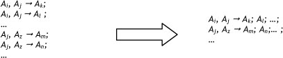
Definition 4. [1,3,4] Fuzzy logical relationships with the same fuzzy set on the left-hand side can be further grouped into a fuzzy logical relationship group. Suppose there are fuzzy logical relationships such that:

then they can be grouped into a fuzzy logical relationship group

Definition 5. [1,3,4] Suppose F(t) is caused by F(t-1) only, and F(t) = F(t-1)xR(t-1, t). For any t, if R(t-1, t) is independent of t, then F(t) is named a time-invariant fuzzy time series; otherwise it is a time-variant fuzzy time series.

Definition 6. [1,3,4] In a multivariate fuzzy inference process, an m-factor /(-order fuzzy time series is a time series consisting of m factors that are of k^th order. For example, a two-factor k^th order fuzzy time series with X as the primary and Y as the second factor could be stated as:

Chen [8] developed a new model based on the above definitions, and simplified Song & Chissom's model. Chen's model provided a better forecasting performance and better integration with heuristic knowledge, compared with Song & Chissom's model [5,8].

However, Chen's model also has a drawback: it omits fuzzy logic relations repetitiveness. To overcome this drawback, this study uses the frequency weighted method [2]. In this case the fuzzy logic relationship (FLR) that occurred often in the past will likely happen often in the future. The procedure of forecasting with fuzzy time series is described as follows:

Step 1. Define the universe of discourse and intervals:

Let the U_mjn and U_max be the minimum and maximum value of historical data, let U = [u_min, u_max] be the universe of discourse. Then U is partitioned into several intervals.

Step 2. Define fuzzy sets based on the intervals, and fuzzify the historical data.

Let U be the universe of discourse, where U={u₁, u₂, u₃, .., u_n}. A fuzzy set A_j is defined by:

where z_Ai is the membership function of fuzzy set A_j, and z_A (u_k) is the degree of belongingness of u_kin A_j. z_A.(u_k)∈[0,1]; 1 <i<m;1 <k<n.

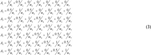
A price or a datum is fuzzified to A₍, if the maximum membership function is under A_{k .} As in the literature, the present study uses a triangular membership function to define fuzzy sets A . To present the procedure here, let the number of intervals be seven. Thus the fuzzy sets are defined by the following equation:

Step 3. Establish fuzzy logical relationships, and group them based on the left hand side. According to Definitions 2 and 3, in first order models the fuzzy relationship F(t-1) -F(t) could be denoted by At - Aj, in which A_i and Aj are the corresponding linguistic values of F(t-1) and F(t) respectively. Therefore, the way of evoking all fuzzy logical relationships under n order is to find any relationship consisting of the type F(t - ή), F(t -n + 1), F(t -η + 2),... F(t- 1) - F(t). Then by replacing the corresponding linguistic values, n order fuzzy relationships were established as At,A¡,Ak ... A¡ - Az.

The FLR with the same left-hand side could establish a FLR group.

Step 4. Assign weights.

All FLRs could establish a fluctuation matrix based on the repetitiveness of each FLR in the historical data. Equation (4) represents a 1χη fluctuation matrix for a specific FLR, in which n denotes the number of fuzzy sets and w¡ 1<i<n indicates the frequency of that specific FLR with the right hand side of A¡ 1<i<n in the historical dataset.

To obtain a frequency weighted matrix, the fluctuation matrix should be standardised by equation (5).

Finally, a frequency weighted matrix for each FLR group is calculated. The weight of a FLR is based on the repetitiveness of that FLR in the past.

Step 5. Calculate the forecast values.

To obtain the forecast value at time t, we will use Eq. (6) where W_n(t-1) is a frequency weighted matrix for a corresponding FLR group of time t-1, and Ldf(t-1) is a deffuzified matrix of fuzzy sets midpoints.

 

4. PROPOSED MODEL

Some studies have shown that intervals of different lengths influence the forecasting accuracy [6,16]. This paper also intends to integrate the SA heuristic with Chen's model to achieve a better performance in forecasting.

4.1 Simulated annealing

Simulated annealing (SA) is an optimisation heuristic that searches the solution space by generating a stochastic neighbourhood. In most heuristics, local optimality is a critical problem. The SA algorithm tries to overcome this problem by accepting bad solutions with a decreasing probability [27,28].

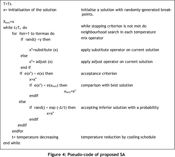
The algorithm starts from a definite initial temperature called (Ts). During the process, temperature (T) decreases gradually by the mechanism of a cooling schedule until it reaches the final temperature (Te). In each iteration the algorithm generates a new solution in the neighbourhood of the current solution. Then by comparing the fitness of the neighbour with the current solution, SA decides whether or not to accept the solution. The algorithm accepts superior neighbours as the current solution; but in the case of inferior- solutions, it accepts the solution by the probability that is generated by the Boltzmann function (-Δ/kT). In this function, k is the constant part, T is the current temperature, and Δ is the difference between the current and the new solution's fitness [27,28].

4.1.1 Encoding scheme

In this section the encoding scheme is described. Let the number of intervals be n, with U_min,U_max as the lower and upper bands of the universe of discourse respectively. The solution X is a vector consisting of n-1 components X = (x₁, x₂,....x_n-1) where x_¿ > x_i_₁ , 1 <i <n- 1. Each element of solution x_¿ is called a break-point. Using this solution, n intervals will be produced as follows: int₁=(U_min, x₁), int₂=(x₁, x₂), ...and int_n=(x_n-1, U_max). Figure 1 is a graphical representation of a solution with seven unequal intervals.

 

 

4.1.2 Neighbourhood search structure

The neighbourhood search structure (NSS) is a procedure that generates a new solution that slightly changes the current solution. A variety of NSSs is available and applied to the SA heuristic algorithm. In order to intensify and diversify the search space, two different NSSs are taken into consideration.

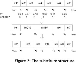
• Substitute operator: the position of randomly chosen break-points regenerated within range (u_min,u_max). In other words, this procedure replaces a randomly-chosen interval with another newly-generated interval. The mechanism of this NSS is a random number (r_i) generated for n-1 break-points. This random number is compared with a constant predefined value (α), if r_¿ > a. The break-point will be replaced by another newly-generated break-point (y_i) where u_min < y_¿ < u_max. Figure 2 is a graphical representation of this procedure in a seven-interval solution where α=0.5.

 

 

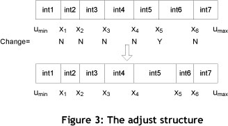
• Adjust operator: the position of a randomly-chosen break-point (x₍) regenerated within the range (max(umin,xi_1) ,min(umax,xi+1) ). In other words, this procedure aims to adjust a randomly-chosen break-point between the previous and the next break-points. The mechanism of this procedure can be explained thus: β is a predefined value that demonstrates the number of break-points that will be adjusted. So randomly-chosen break-points (x_i) will be replaced with new break-points where max(umin,xt-1) < yt < min(umax,xi+1) . Figure 3 is a sample graphical representation of Adjust operator on a seven-interval solution where β=1.

 

 

• Mix operator: Finally, these two operators - one of which tries to diversify (substitute), while the other tends to intensify (adjust) the search space - must be combined, with the third operator used as a mixer. The mechanism of this operator is thus: A random number (r) is generated and compared with a predefined value such as ye [0,1]. If r < γ the substitute operator will apply to the current solution; otherwise the adjust operator will be applied.

4.1.3 Cooling schedule

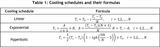
The main goal of using a cooling schedule is to control the SA heuristic's behaviour. As explained above, to avoid becoming trapped in local optimums, the SA heuristic accepts a worse solution using a probability that is generated by the Boltzman function. This probability depends on a temperature that decreases steadily by a mechanism called a cooling schedule. There are three types of cooling schedule in the literature: linear, exponential, and hyperbolic. Table 1 presents the formula and the procedure of each mechanism, where Ts¡ Te¡ and N are the starting temperature, the stopping temperature, and the number of temperatures between T_s and T_e respectively. By conducting some initial experiments, linear and exponential cooling schedules result in the proposed model's better performance. Following the procedure described in [29], the starting temperature over the range 4 to 10 is appropriate for the problem; the stopping temperature is also determined over the range 0.001 to 0.1.

 

 

4.1.4 Boltzman function

In order to define the Boltzman function it is necessary first to determine the objective function of the model. The objective of forecasting models is to reduce forecasting errors. There are different ways of calculating error in the literature. One of these methods, which is prevalent in the literature, is the mean square error (MSE) [16]. E(x) indicates the forecasting error of solution X, which is calculated by a definition of MSE as follows:

in which n denotes the number of forecasted data, F_i denotes the ith forecasted data, and A_i denotes the actual corresponding data. The function is often taken to be a Boltzman function, in which E(Xⁿ), E(X^c), T_i, denotes a new solution error, a current solution error, and the temperature at ith iteration respectively.

The MSE performance measure depends on the amount of forecasted data. In order to handle different test problems with different ranges of data, a dimensionless Boltzman function is needed; therefore, AE is defined as:

4.2 Parameter calibration

There are parameters in the SA heuristic that need to be tuned, as each of them has an effect on the algorithm's performance. Therefore, designing parameters appropriately makes them more efficient - depending, of course, on the nature of the problem. It is important to know that when a model or problem changes, the parameters must change. According to the literature, many researchers do not apply any tuning method to their problems. This study aims to design an experimental test to tune all parameters.

There are so many approaches to the design of experimental tests. The most widely used -and comprehensive - method is full factorial. However, it is extremely time-consuming in problems with a large number of parameters, such as those included in this study, because the method examines every possible combination of factors. For that reason, fractional factorial experiments (FFE) were developed [30] to reduce the required number of experimental tests. The Taguchi method uses the orthogonal array to investigate the combination of factors and to measure the main effect of each one by designing a small number of experimental tests [31].

Taguchi divides factors into two basic groups: controllable and noise (uncontrollable) factors.

There is no direct control over noise factors. The Taguchi method is used to minimise the effect of the noise factors, and to set the optimum level of the controllable factors, based on the concept of robustness [32]. The Taguchi method also demonstrates the relative significance of each factor in its impact on the objective function.

A transformation of the repetition data to another value is the measure of variation developed by Taguchi. Because of this transformation, which produces a signal-to-noise ratio (S/N), the Taguchi method is considered to be a robust design [32]. In this method, the terms 'signal' and 'noise' indicate the desirable value (response variable) and undesirable value (standard deviation) respectively. The method tends to maximise the signal-to-noise ratio.

In this method, objective functions have been divided into three main groups: the-smaller-the-better, the-larger-the-better, and nominal-is-best. Since our forecasting objective function is classified as 'the-smaller-the-better', the corresponding signal-to-noise ratio [32] is:

For this problem, eight factors are considered to be SA control factors: cooling schedule, starting temperature, stopping temperature, value of desired temperature, value of neighbourhood search in each temperature, substitute operator parameter (α), adjust operator parameter (β) and mix operator (y). Table 2 sets out the controllable factors and their related levels.

 

 

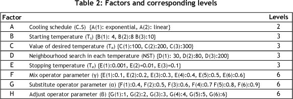
The cumulative degree of freedom for these factors is 24, so the appropriate orthogonal array for this problem should have at least 24 rows and 8 columns. For the orthogonal array in this case, two modifications need to be done. First, the omission of two columns with three levels is necessary.

Second, a two-level factor of the case (factor A: cooling schedule) lacks one level compared with L₃₆. To offset this gap, one optionally selected existing level of the related factor needs to be allotted to that extra level. So the third level of factor A is set as a repetition of level 1. Table 3 shows 36 experimental tests that were designed according to the modified L36.

 

 

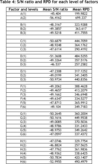
Taguchi-designed experiments are conducted using a three-order fuzzy time series model on the Alabama University enrolment as a prominent test problem in the area of fuzzy time series. To get more reliable information, each trial is implemented three times. In all the experiments, Matlab 7.1 is used on a PC with a 2.4 GHz Intel Core 2 Duo processor and 4 GB of RAM. In order to compare the experimental tests, relative percentage deviation (RPD) is used as a performance measure, calculated as follows:

where min_sol is the best result obtained for a given test problem among the experimental trials, and trial_sol is the objective value (MSE) obtained in an experimental trial.

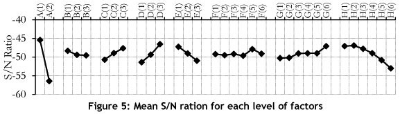
The results obtained for each experiment were transformed into a S/N ratio. Figure 4 shows the average S/N ratio for each level. As shown in Figure 5, A(1), B(1), C(3), D(3), E(1), H(2) are the optimum levels of factors A, B, C, D, E, H respectively. Determining the optimal level of factors F and G needs more investigation, for which, the RPD needs to be analysed.

 

 

 

 

The results of the average RPD are shown in Figure 6. This analysis strongly confirmed the optimal levels for factors A, B, C, D, E, and H, and it was found that F(4) and G(4) were the superior levels, with a minimum RPD for factors E and F respectively. Thus the chosen levels are as follows:

 

 

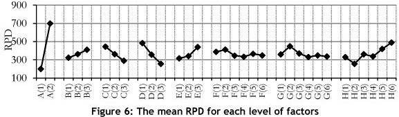
• Cooling schedule: exponential, starting temperature: 4.
• Value of desired temperature: 300.
• Neighbourhood search in each temperature: 200.
• Stopping temperature: 0.001.
• Mix operator parameter: 0.4.
• Substitute operator parameter: 0.7.
• Adjust operator parameter: 2.

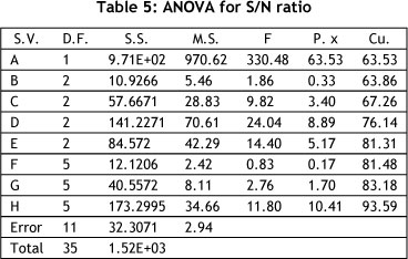
To examine the relative significance of the factors in terms of their impact on the objective function, an analysis of variance (ANOVA) was applied to the S/N ratio. The results are given in Table 4. The cooling schedule (A) factor has the largest impact on the objective function with a relative significance of 63.53%. After this factor, the next most important ones were: adjust operator parameter (H), at 10.41%; neighbour search in each temperature (D), 8.89%; stopping temperature (E), 5.17%; and number of desired temperature (C), 3.40%. The remaining factors - B, F, and G - had the least impact on the quality of the objective function.

 

 

 

 

5. EXPERIMENTAL EVALUATION

The proposed model was applied to the Alabama University enrolment data. A comparison of the results from the proposed model, from Kuo et al. [16], and from Chen & Chung [14], based on the different number of intervals and first-order forecasting, is shown in Table 6.

 

 

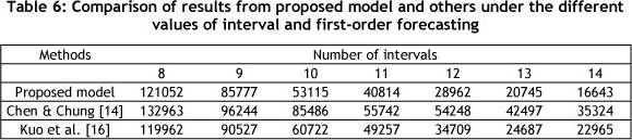
The main difference between the three methods is the heuristic algorithms that were used to forecast. Chen & Chung [14] used the genetic algorithm; Kuo et al. [16] used the PSO heuristic; while this study has proposed a method that benefits from the SA heuristic algorithm. This model is well-tuned by the Taguchi orthogonal arrays method. From Table 7 it is clear that the proposed model offers a better performance in achieving the appropriate set of intervals.

 

 

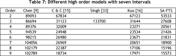
In the next step, a comparison is carried out between the proposed model and existing high-order models. The results are given in Table 7. They clearly indicate that the proposed model offers the greatest accuracy among all existing models.

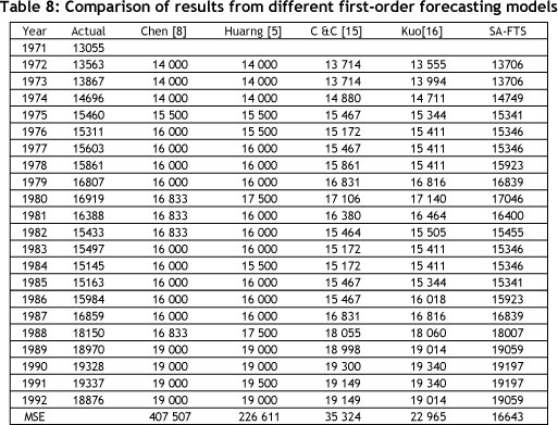
Table 8 contains a comparison of the forecasted enrolments generated by the proposed model and existing first-order fuzzy time series, with different number of intervals, such as Chen [8], Huarng [5], Chen & Chung [15] and Kuo et al. [16]. Three of the models - Chen & Chung [15], Kuo et al. [16], and the proposed model - used first order fuzzy forecast rules and 14 intervals to forecast enrolments.

 

 

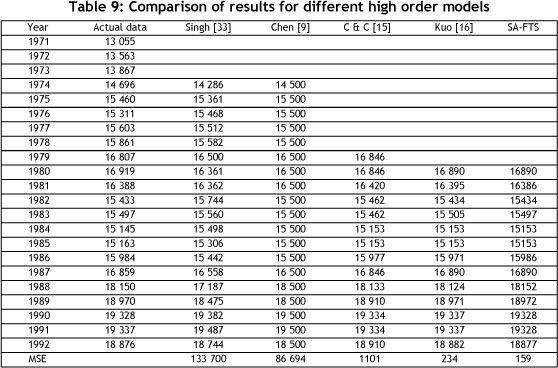
As the final step, the proposed model was compared with other high-order fuzzy forecasting models such as Chen [9], Singh [33], Chen & Chung [15], and Kuo et al. [16]. The results are shown in Table 9, where two of the models [15, 16] and the proposed model use ninth-order fuzzy rules and 14 intervals to forecast enrolments.

 

 

All of the experimental results clearly confirmed that the new proposed SA is superior to the other algorithms in its different fuzzy order rules and number of intervals.

 

6. CONCLUSION

This paper dealt with a new forecasting model based on the simulated annealing (SA) heuristic and fuzzy time series (FTS) to forecast the Alabama University's enrolment dataset. The proposed metaheuristic struck a compromise between intensification and diversification by using two neighbourhood search structures called 'adjust' and 'substitute' operators. To enhance the quality of the simulated annealing, a comprehensive comparison has been made between different parameters of the algorithm to obtain their precise calibration by means of the Taguchi method. To investigate the model's effectiveness in comparison with other models in the literature, the experimental results revealed the superiority of the proposed simulated annealing based model (SA-FTS).

The SA-FTS was tested on Alabama enrolments under one factor condition. It could be applied to other problems with two or more factors, such as temperature prediction and stock indices, in further research.

 

REFERENCES

[1] Song, Q. & Chissom, B.S. 1993. Forecasting enrollments with fuzzy time series - Part I, Fuzzy Sets and Systems, 54 (1), pp 1-9.         [ Links ]

[2] Tsaur, R.C., Yang, J.C. & Wang, H.F. 2005. Fuzzy relation analysis in fuzzy time series model, Computers and Mathematics with Applications, 49 (4), pp 539-548.         [ Links ]

[3] Song, Q. & Chissom, B.S. 1993. Fuzzy time series & its models, Fuzzy Sets & Systems, 54 (3), pp 269-277.         [ Links ]

[4] Song, Q. & Chissom, B.S. 1994. Forecasting enrollments with fuzzy time series - Part II, Fuzzy Sets & Systems, 62 (1), pp 1-8.         [ Links ]

[5] Huarng, K. 2001. Heuristic models of fuzzy time series for forecasting, Fuzzy Sets & Systems, 123 (3), pp 369-386.         [ Links ]

[6] Huarng, K. 2001. Effective lengths of intervals to improve forecasting in fuzzy time series, Fuzzy Sets & Systems, 123, pp 387-394.         [ Links ]

[7] Zadeh, L.A. 1965. Fuzzy sets, Information & Control, 8, pp 338-353.         [ Links ]

[8] Chen, S.M. 1996. Forecasting enrollments based on fuzzy time series, Fuzzy Sets & Systems, 81 (3), pp 311-319.         [ Links ]

[9] Chen, S.M. 2002. Forecasting enrollments based on high-order fuzzy time series, Cybernetics & Systems: An International Journal, 33, pp 1-16.         [ Links ]

[10] Jilani, T.A. 2007, Fuzzy metric approach for fuzzy time series forecasting based on frequency density based partitioning, in World Academy of Science, Engineering & Technology Conference.         [ Links ]

[11] Cheng, C.H. 2008. Fuzzy time-series based on adaptive expectation model for TAIEX forecasting, Expert Systems with Applications, 34, pp 1126-1132.         [ Links ]

[12] Lee, L.W., Wang, L.H. & Chen, S.M. 2007. Temperature prediction & TAIFEX forecasting based on fuzzy logical relationships & genetic algorithms, Expert Systems with Applications, 33 (33), pp 539-550.         [ Links ]

[13] Lee, L.W., Wang, H.F. & Chen, S.M. 2008. Temperature prediction & TAIFEX forecasting based on high-order fuzzy logical relationships & genetic simulated annealing techniques, Expert Systems with Applications, 34 (1), pp 328-336.         [ Links ]

[14] Chen, S.M. & Chung, N.Y. 2006. Forecasting enrollments of students by using fuzzy time series & genetic algorithms, International Journal of Information & Management Sciences, 17, pp 1-17.         [ Links ]

[15] Chen, S.M. & Chung, N.Y. 2006. Forecasting enrollments using high-order fuzzy time series & genetic algorithms: Research Articles, International Journal of Information & Management Sciences, 21, pp 485-501.         [ Links ]

[16] Kuo, H., Horng, H., Kao, S.J., Lin, T.W., Lee, T.L. & Pan, C.L. 2009. An improved method for forecasting enrollments based on fuzzy time series & particle swarm optimization, Expert Systems with Applications, 36, pp 6108-6117.         [ Links ]

[17] Park, J.I., Lee, D.J., Song, C.K. & Chun, M.G. 2010. TAIFEX & KOSPI 200 forecasting based on two-factors high-order fuzzy time series & particle swarm optimization, Expert Systems with Applications, 37, pp 959-967.         [ Links ]

[18] Yolcu, U., Egrioglu, E., Uslu, V.R., Basaran, M.A. & Aladag, C.H. 2009. A new approach for determining the length of intervals for fuzzy time series, Applied Soft Computing, 9 (2), pp 647651.         [ Links ]

[19] Chu, H.H., Chen, T.L., Cheng, C.H. & Huarng, C.C. 2009. Fuzzy dual factor time-series for stock index forecasting, Expert Systems with Applications, 36 (1), pp 165-171.         [ Links ]

[20] Cheng, C.H., Chen, Y.S. & Wu, Y.L. 2009. Forecasting innovation diffusion of products using trend-weighted fuzzy time-series model, Expert Systems with Applications, 36 (2), pp 1826-1832.         [ Links ]

[21] Wang, N.Y. & Chen, S.M. 2009. Temperature prediction & TAIFEX forecasting based on automatic clustering techniques & two-factors high-order fuzzy time series, Expert Systems with Applications, 36 (2), pp 2143-2154.         [ Links ]

[22] Teoh, H.J., Cheng, C.H., Chu, H.H. & Chen, J.S. 2008. Fuzzy time series model based on probabilistic approach & rough set rule induction for empirical research in stock markets, Data & Knowledge Engineering, 67 (1), pp 103-117.         [ Links ]

[23] Leu, Y., Lee, C.P. & Jou, Y.Z. 2009. A distance-based fuzzy time series model for exchange rates forecasting, Expert Systems with Applications, 36 (4), pp 8107-8114.         [ Links ]

[24] Egrioglu, E., Aladag, C.H., Yolcu, U., Basaran, M.A. & Uslu, V.R. 2009. A new hybrid approach based on SARIMA & partial high order bivariate fuzzy time series forecasting model, Expert Systems with Applications, 36 (4), pp 7427-7434.         [ Links ]

[25] Bahrepour, M., Akbarzadeh-T, M.R., Yaghoobi, M. & Naghibi-S, M.B. 2011. An adaptive ordered fuzzy time series with application on FOREX, Expert Systems with Applications, 38 (1), pp 475485.         [ Links ]

[26] Liu, H.T. & Wei, M.L. 2010. An improved forecasting method for seasonal time series, Expert Systems with Applications, 37 (9), pp 6310-6318.         [ Links ]

[27] Kirkpatrick, S., Gellat, C.D. & Vecchi, M.P. 1983. Optimization by simulated annealing, Science, 220 (4598), pp 671-680.         [ Links ]

[28] Metropolis, N., Rosenbluth, A.W., Rosenbluth, M.N., Teller, A.H. & Teller, E. 1953. Equations of state calculations by fast computing machines, Journal of Chemical Physics, 21, pp 1087-1092.         [ Links ]

[29] Crama, Y. & Schyns, M. 2003. Simulated annealing for complex portfolio selection problems, European Journal of Operational Research, 150, pp 546-571.         [ Links ]

[30] Cochran, W.G. & Cox, G.M. 1992. Experimental designs, 2^nd edition. Wiley.         [ Links ]

[31] Ross, R.J. 1989. Taguchi techniques for quality engineering. McGraw-Hill.         [ Links ]

[32] Phadke, M.S. 1989. Quality engineering using robust design. Prentice-Hall.         [ Links ]

[33] Singh, S.R. 2007. A simple method of forecasting based on fuzzy time series, Applied Mathematics & Computation, 186, pp 330-339.         [ Links ]

 

 

* Corresponding author.