CASE STUDIES

 

Coordinated location, distribution and inventory decisions in supply chain network design: a multi-objective approach

 

 

G. Reza Nasiri^{I, *}; Hamid Davoudpour^II

^IDepartment of Industrial Engineering Amirkabir University of Technology, Tehran, Iran. reza_nasiri@aut.ac.ir
^IIDepartment of Industrial Engineering Amirkabir University of Technology, Tehran, Iran. hamidp@aut.ac.ir

 

 

---

ABSTRACT

This research presents an integrated multi-objective distribution model for use in simultaneous strategic and operational food supply chain (SC) planning. The proposed method is adopted to allow use of a performance measurement system that includes conflicting objectives such as distribution costs, customer service level (safety stock holding), resource utilisation, and the total delivery time, with reference to multiple warehouse capacities and uncertain forecast demands. To deal with these objectives and enable the decision makers (DMs) to evaluate a greater number of alternative solutions, three different approaches are implemented in the proposed solution procedure. A detailed case study derived from food industrial data is used to illustrate the preference of the proposed approach. The proposed method yields an efficient solution and an overall degree of DMs' satisfaction with the determined objective values.

---

OPSOMMING

Die navorsing behandel 'n geïntegreerde multidoelwit distribusiemodel vir strategiese beplanning van 'n voedseltoevoerketting. Om met die model doelmatig te werk, moet 'n versameling van randvoorwaardes hanteer word om die saamgestelde optimiseringsdoelwit te bereik teen 'n agtergrond van uiteenlopende sienings.

---

 

 

1. INTRODUCTION

The distribution planning decision (DPD) is one of the most comprehensive strategic decision issues that need to be optimised for the long-term efficient operation of a whole supply chain (SC). The DPD involves optimising the transportation plan for allocating goods and/or services from a set of sources to various destinations in a supply chain (Liang [1]). An important strategic issue related to the design and operation of a physical distribution network in a supply chain system is the determination of the best sites for intermediate stocking points, or warehouses. The use of warehouses provides a company with flexibility to respond to changes in the marketplace, and can result in significant cost savings due to economies of scale in transportation or shipping costs.

The major task of DPD is the determination of distribution costs, customer service level (safety stock holding), resource (warehouse space) utilisation, and the total delivery time, with reference to multiple warehouse capacities and uncertain forecast demands (Torabi & Hassini [2]).

In previous studies, both deterministic and stochastic customers' demands have been considered, but more attention has been paid to the deterministic cases. (See the recent survey on stochastic components in facility location models by Snyder [3].)

Generally, the applied constraints in modelling DPDs are the capacity limitation and single source constraints (Farahani & Elahipanah [4]). In some cases, in addition to the capacity constraints, some other restrictions on the number of covered demands and the service levels of the warehouses are also defined.

Recently some authors have incorporated inventory control decisions into DPD models. For example, Miranda & Garrido [5, 6], Daskin et al. [7], and Shen et al. [8] present similar versions of the DPD model incorporating the inventory control decisions.

Erlebacher & Meller [9] present a location-inventory model for designing a two-level distribution system serving continuously represented customer locations. They develop a stylised analytical model to provide some intuition and basic results for the problem. The stylised model also motivates bounds for the problem, which they use to develop a heuristic. They show that the heuristic performs very well on test problems that considered variation in customer demand and spatial dispersion.

In these works, the ordering decisions are based on the classic economic order quantity (EOQ) model, and a normal distribution is assumed for the demand pattern.

Additionally, researchers have developed various methods to solve multi-objective DPD problems. Liang [1] develops an interactive fuzzy multi-objective linear programming method for solving the fuzzy multi-objective DPD problem with piecewise linear membership functions. Selim & Ozkarahan [10] suggest an interactive fuzzy goal programming (FGP) for the supply chain distribution network design. The goal of their model is to select the optimum numbers, locations, and capacity levels of the plants and warehouses to deliver the products to the retailers at the least cost while satisfying the preferred customer service level.

In most of the past research studies like Gourdin et al. [11], Jayaraman [12], Pirkul & Jayaraman [13], and Tragantalerngsak et al. [14], one major drawback is that they limit the number of capacity levels available to each facility to just one. However, in real case studies, there are usually several capacity levels to choose for each facility. This flexibility in capacity levels makes the problem more realistic and, at the same time, more complex to solve. Another major drawback in some previous studies is that they limit the number of opening facilities to a pre-specified value. Moreover, these studies fail to describe how this value can be determined in advance. Amiri [15] represents a significant improvement over previous research by presenting a unified model of the problem that includes the numbers,- locations, and capacities of both warehouses and plants as variables to be determined in the model. In addition, he develops an efficient heuristic solution procedure based on Lagrangean Relaxation (LR) of the problem, and reports extensive computational tests with up to 500 customers, 30 potential warehouses, and 20 potential plants.

In this paper we develop a new non-linear multi-objective DPD model, consisting of one manufacturer and multiple distribution centres (warehouses), that integrates the location/allocation and distribution plans. In this model, to improve over previous research, we also incorporate tactical/operational decisions - such as inventory control decisions -into the DPD problem. Then we propose an efficient goal programming approach to solve the developed model. We consider three important objective functions:

• investment in opening distribution centres/warehouses (location costs);
• total cost of logistics, such as the costs of transporting products from the plant to the opened warehouses, and from the opened warehouses to the retailers, and holding costs (inventories and safety stocks); and
• total delivery time.

The problem is particularly motivated by consulting work that was done for a large food industry company owning one production site and multiple distribution centres. Since the transportation cost constitutes the main part of the unit cost, and since delivery time and limited storage capacity are also very important, implementing the distribution planning system for the DCs' location and inventory control decisions is of particular interest.

The paper has two important applied and theoretical contributions. First, it presents a new comprehensive and practical, but tractable, optimisation model for distribution network designing. Second, it introduces a novel solution procedure for finding more non-dominated and efficient compromise solutions to a stochastic multi-objective mixed-integer programme. In our literature survey we have found a lack of studies in this field, which is understandable, given that large mixed integer programming is known to be complex even when all data is certain and precise.

The remainder of this paper is organised as follows. In Section 2 we consider a summary of key challenges in agro-food supply chains. In Section 3 we define our notation, state our assumptions, and propose a new multi-objective stochastic non-linear program (MOSNLP) for the proposed DPD problem. After applying appropriate strategies for converting the stochastic model into a multi-objective nonlinear model (MONLP), in Section 4 we propose a novel interactive payoff approach to solve this MONLP and find an efficient compromise solution. The proposed model and the solution method are validated through numerical tests in Section 5. The data for these numerical computations have been inspired by a real life food industrial case study, as well as randomly generated data. Concluding remarks on computational results and further research directions are the subject of Section 6.

 

2. IMPORTANT PROBLEMS IN SUPPLY CHAIN MANAGEMENT IN THE FOOD SECTOR

Almost without exception, all well-known industries are redesigning their distribution networks in a bid to meet global trends and continue to meet customer demands. Considering the competitive market, key food industries must work on the optimal supply chain structure. However there is no doubt that supply chain networks are confronting new challenges. Hunt et al. [16] summarise these challenges:

• More instances of multi-site manufacturing
• Increasingly cut-throat marketing channels
• The maturation of the world economy
• Heightened demand for local products
• Competitive pressures to provide exceptional customer service
• Quick, reliable delivery
• Commonality of turbulence and volatility in markets
• Time-to-market for new products

Based on these challenges, in this paper we focus on supply chain costs, customer service level, and delivery time in food distribution planning.

 

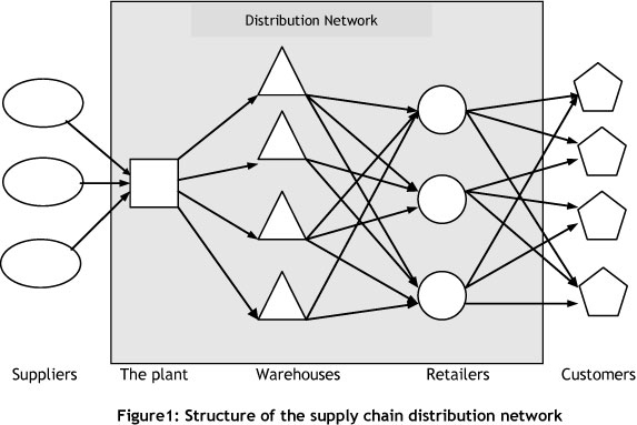
3. PROBLEM SCOPE AND FORMULATION

We consider a firm that owns a manufacturing plant that is capable of producing multiple products. The products are then delivered to different distribution centres (warehouses/wholesalers) in order to satisfy their associated dynamic demands. The network is illustrated in Figure 1.

 

 

Assume that in the company the logistics centre seeks to determine the right transportation plan to allocate multiple commodities from the source (factory) to J warehouses (DCs). Each destination has a forecast demand of each commodity to be received from the plant. The forecast demand of each warehouse depends on uncertain demands of allocated customers to this warehouse. This work focuses on developing a MOSNLP method to optimise distribution decisions such as location/allocation and inventory policy in a food industry company.

This problem in fact integrates three decision sub-problems: (1) selecting the optimum numbers, locations, and capacity levels of the warehouses to deliver products to retailer/customer at the least cost while satisfying desired service level to retailers; (2) allocation of these retailers to the open warehouses; and (3) inventory decisions for the supply chain.

Decision-making in such a complex supply chain network requires the consideration of conflicting objectives and of different constraints imposed by the manufacturer and distributors. Moreover, in practical situations, due to the variability and/or uncertainty of required data over the strategic and mid-term horizon, most of the parameters embedded in a DPD problem are frequently stochastic in nature, and can be obtained through probabilities or subjectively in a fuzzy environment. For example, in a real decision problem, market demands, cost/time coefficients, and the amounts of available resources are usually imprecise over the planning horizon, and therefore assigning a set of crisp values for such ambiguous parameters is not appropriate. We rely on probability theory to model this uncertainty. This theory uses statistical distributions to handle this inherently ambiguous phenomenon in the problem parameters.

3.1 Problem description, assumptions, and notation

The stochastic multi-objective DPD problem examined here can be described as follows:

• In the analysed case study, the plant location is known and fixed. The network considered encompasses a set of retailers with known locations, and a discrete set of possible location zones/sites where the plant and warehouses are located.
• The final products have stochastic retailer demand over the given finite planning horizon with mean d_il and variance v_il (note that our customers are mostly retailers, not end consumers).
• There are multiple values for storage capacity at each warehouse (five level storage capacities).
• The distribution costs and delivery time on the given route are directly proportional to the shipped units.
• Products are independent of each other, related to marketing and sales price.
• The number of potential DCs and their maximum capacities are known.
• Retailers receive each product only from a single DC.
• No inventory is held in the plant.
• Decisions are made within a single period.

The indices, parameters, and variables used to formulate the mathematical problem are described as follows:

Indices:

I            index set of customers/customer zones (i=1,....., I)

J            index set of potential warehouse sites (j=1,....,J)

L            index set of products (l=1,...,L)

H            index set of capacity levels available to the potential warehouses (h=1,_,H)

G            index for objectives for all g=1,2,3

η             investment cost performance index [0,1]

γ             delivery time performance index [0,1]

K            customer service performance index [0,1]

Z_l-a        normal distribution value for system service level

Parameters:

TCjjt       unit cost of supplying product l to customer zone i from warehouse on site j

      unit cost of supplying product l to warehouse on site j from the plant

t_ijl          delivery time per unit delivered from warehouse j to customer zone i for each product l

t_ij           delivery time per unit delivered from the plant to warehouse j for each product l

LTj'j        the elapsed time between two consecutive orders of product l for site j

Ρ             fixed cost for opening and operating warehouse with capacity level h on

F_jh          site j per time unit

d_il           mean demand of product l from customer zone i per time unit

v'_il          variance demand of product l from customer zone i per time unit

HC_jl         holding cost of product l in warehouse on site j per time unit

OC_jt        ordering cost of product l from warehouse on site j to the plant

cap_jh       capacity of warehouse on site j with capacity level h

s_t            space requirement of product l at any warehouse

PH            planning horizon

Decisions variables:

X_jh           it takes value 1, if a warehouse with capacity level h is installed on potential site j, and 0 otherwise;

D_ij            it takes value 1, if the warehouse on site j serves product l of customer i, and 0 otherwise;

Dji           mean demand of product l to be assigned to warehouse on site j per time unit

V_jl'          variance demand of product l to be assigned to warehouse on site j per time unit

3.2 Stochastic multi-objective non-linear programming model

3.2.1 Objective functions

We have selected the multi-objective functions for solving the DPD problem by reviewing the literature and considering practical situations. In particular, these objective functions are normally stochastic or fuzzy in nature owing to incomplete and/or uncertain information over the planning horizon. Accordingly, three objective functions are simultaneously considered in formulating the original stochastic DPD problem, as follows:

• Minimise total investment (INV) in opening DCs/warehouses:

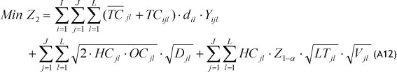
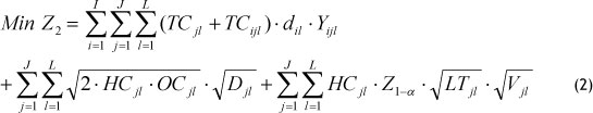
• Minimise total costs (TCOST)

This objective function contains (see Appendix):

• Transportation cost of products from the plant to the warehouses and from the warehouses to the retailers
• Holding cost for mean inventory and safety stocks

• Minimise total delivery time (TDELT)

3.2.2 Constraints

• Constraints that ensure that each retailer is served exactly for each product by one warehouse (single source):

• Constraints of the warehouse capacity:

• Constraints that compute the served average demand by each warehouse:

• Constraints that indicate the total variance of the served demand by each warehouse:

Implicitly, we assume that the demands are independently distributed across the retailers, and thus that all the covariance terms are zero.

• Constraints that ensure that each warehouse can be opened at least at one capacity level

• Binary constraints of decision variables:

 

4. THE PROPOSED SGP-BASED SOLUTION APPROACH

4.1 Defining the goals of the objective functions

As we know, stochastic goal programming (SGP) needs an aspiration level for each objective. These aspiration levels are determined by DMs. In addition to the aspiration levels of the goals, we need max-min limits (u_g , l_g) for each goal. While the DMs decide the max-min limits, the linear programming results are starting points, and the intervals are covered by these results. Note that in non-linear programming (with a minimisation objective) the minimum limit of any non-linear objective may be calculated by the results of the other objectives. This situation may occur because the optimum value may be its local optimum.

Generally the DMs find estimates of the upper (u) and lower (l) values for each goal using payoff table (Table 1). Thus the feasibility of each stochastic goal is guaranteed [10].

 

 

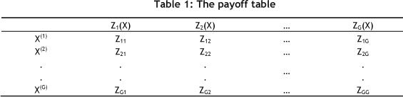
Here, Z_g(X) denotes the gth objective function, and X^(g) is the optimal solution of the gth single objective problem. Solving the problem with X^(g) (g=1,...,G) for each objective, a payoff matrix with entries Z_pg =Z_g (X^(p)), g, p=1,...,G can be formulated as presented in Table 1. Here, u_g= max (Z_1g, Z_2g, . . . , Z_Gg) and l_g=Z_gg , g =1,..., G.

Using the interactive paradigm can improve the flexibility and robustness of multi-objective decision making by:

• Providing a learning process about the system, whereby the DMs can learn to recognise good solutions,
• The DMs can control the search direction during the solution procedure and, as a result, the efficient solution achieves their preferences,
• Various scenarios could be generated, based on a systematic procedure.

4.2 Solution methodology

To deal with multi-objectives and enable the DMs to evaluate a greater number of alternative solutions, three different approaches are implemented in this section.

Solution Approach 1. The weights of objective Z₁ and Z₂ are specified with W₁ and W₂ as follows:

Note that, based on the three presented objective functions and preferred DMs' service level (K), in this approach we generate several scenarios and the TDELT objective is not considered. (A more detailed explanation about the service level of the system is presented in Appendix) So problem 1 can be summarised as follows:

Generated Problem 1

TH allows one to sum the investment cost that occurs at the beginning of the planning horizon with the rate cost incurred by the entire network. In order to determine the weights, there are some good approaches in the literature, such as the analytical hierarchy process, the weighted least square method, and the entropy method. However, determination of the weights is not the focus of this study.

Solution Approach 2. In this approach the weights of the objectives ( Z1, Z2 ) and preferred DMs' service level are the same as in solution approach 1, but we consider Z₃ (TDELT objective) as a new constraint.

Generated Problem 2

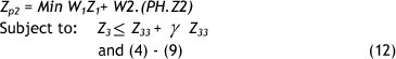
In the payoff table we calculate optimum (or local optimum) values for the three objective functions. In this approach, to compare each objective function against the others, we use the performance Index as a compensation rate. Since objectives Z₃ and Z₂ are very interactive, it is important for the DMs to evaluate the impact of increasing γ % in total delivery time (TDELT) on the system costs (INV and TCOST). To generate new scenarios we calculate the γ parameter based on the DMs preferences.

Solution Approach 3. In this approach, the objective function is TCOST and the other objectives (INV, TDELT) are added to the previous constraints (4)-(9). As in solution approach 2, it is important for DMs to consider Z₁ and Z₃ against the TCOST objective function.

Generated Problem 3:

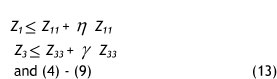
To generate more scenarios we calculate η and γ parameters based on the DMs preferences.

4.3 Solution procedure

The interactive solution procedure of the proposed MOSNLP method for solving stochastic multi-objective DPD problems includes the following steps:

Step 1 : Formulate the original stochastic MOSNLP model for the DPD problem.

Step 2: Obtain efficient extreme solutions (payoff values) used for constructing the right-hand side of the added constraints (first and third objective functions). If the DMs select one of them as a preferred solution, go to Step 10.

Step 3: Define upper and lower bounds of each objective functions from the payoff table.

Step 4: Formulate problems 1, 2 and 3.

Step 5: Ask the DMs if they want to modify the right-hand side of the newly-added constraints of problems 2 and 3.

Step 6: Introduce η and γ parameters to generate new scenarios - i.e., define a systematic rule for changing upper bound of Z₁ and Z₃

Step 7: Determine the values of the SC performance vector (W₁ , W₂, η, γ, K).

Step 8: Improve the generated scenarios with the performance vector determined in Step 7.

Step 9: Analyse outputs of generated scenarios and obtain non-dominated solutions. If the DMs select one of them as a preferred solution, go to Step 10; otherwise, go to Step 5.

Step 10: Stop.

 

5. CASE STUDY

The case study presented here, with an example from the food industry, illustrates the algorithm proposed in Section 4, as well as the applicability and effectiveness of the model. This food industry company is the leading producer of two main categories of Iranian food and drink (rice and tea). The basic distribution data are presented in the next sub-section.

5.1 Setup

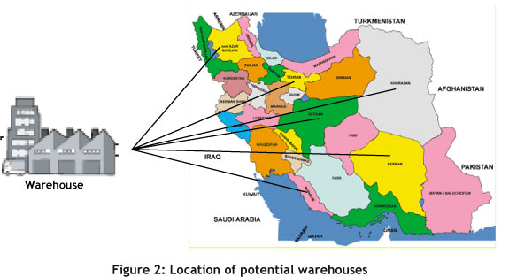
A case study inspired by a food producer in Iran is presented to demonstrate the validity and practicality of the model and solution method. The company owns one production site and six potential DC/warehouse sites in the different customer zones (Figure 2). There are three types of products and twenty main retailers.

 

 

Lingo 8.0 optimisation software is used as the problem solver. All scenarios are solved on a Pentium 4 (Core 2 Duo) with 1GB RAM and 4 GHz CPU.

Because of confidentiality, the input data are randomly generated. However, the generation process is done so that it will be close to the real data available in the company. Without loss of generality and just to simplify generation of the stochastic parameters, we apply the pattern of a systematically normal distribution for our numerical test.

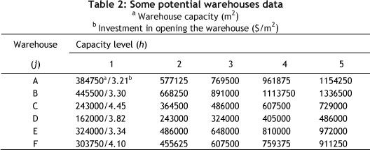
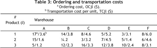
The required throughput capacity of any warehouse for product ' is as follows: s_,= 2, s₂= 5, s₃= 4. Tables 2 and 3 list some of the other basic distribution data.

 

 

 

 

5.2 Performance analysis

The interactive solution procedure using the proposed SGP method for the case study is as follows:

First, formulate the original stochastic multi-objective DPD problem according to equations (1)-(9). The goal of the model is to select the optimum numbers, locations, and capacity levels of warehouses to deliver the products to the retailers at the least cost, while satisfying the desired service level of the retailers. The proposed model is distinguished from the other models in this field in the modelling approach. Because of the somewhat uncertain nature of retailers' demand and DMs' aspiration levels for the goals, a stochastic modelling approach is used. Additionally, a novel and generic SGP-based solution approach is proposed to determine the preferred compromise solution.

Second, obtain efficient extreme solutions for each of the objective functions. These extreme solutions of the case study are presented in Table 4.

 

 

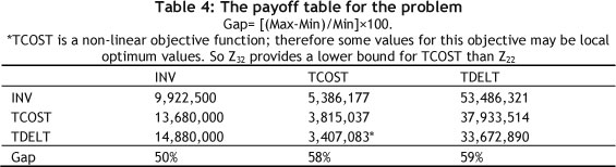
It is assumed that the DMs do not choose any of the efficient extreme solutions as the preferred compromise solution, and proceed to the next step.

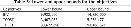
Considering the efficient extreme solutions given in Table 4, the lower and upper bounds of the objectives can be determined. In our case, the corresponding minimum and maximum values of the efficient extreme solutions are determined as the lower and upper bounds respectively, as presented in Table 5.

 

 

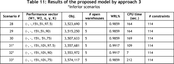
After calculating the upper and lower bounds of each objective function, the next step is formulation of problems 1, 2 and 3. A summary of the results for the various scenarios is given in Tables 6, 9 and 11.

 

 

 

 

 

 

 

 

 

 

 

 

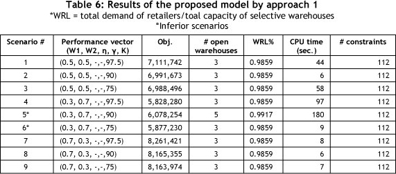
As stated previously, the relative weights for the first and second objective functions in problem 1 can be determined by DMs using various methods. For the presented case study, DMs determine three weights for the INV and TCOST objectives as follows: (0.7, 0.3), (0.5, 0.5) and (0.3, 0.7). For this problem, no constraint on delivery time is included and TH=1000 (planning horizon) hereafter. By fixing the values of W1 and W₂, the solution given in Table 6 is obtained. In this table, for three values of each objective function and three levels for the customer service performance index (K), nine scenarios have been generated.

In Table 6, the warehouse load ratio percentage (WRL) column shows the efficiency of the opened warehouses. The average WRL in approach 1 is 0.9865, and since Z_p1 is a non-linear objective function, the range of the CPU time for solving this problem is very wide, from 6 to 180 seconds.

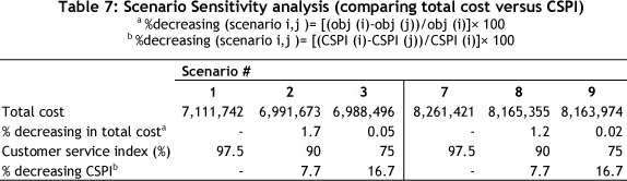
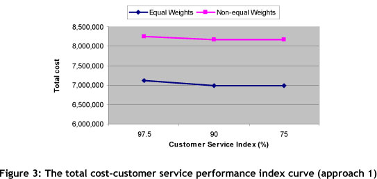
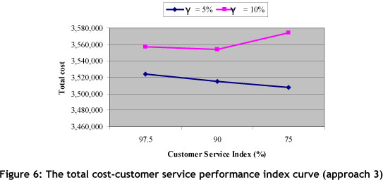
Note that in scenarios 5 and 6, although the customer service performance (90%, 75%) is lower than in the 4^th scenario (97.5%), the objective function is higher. Therefore these scenarios are inferior and must be removed from the scenario list. Figure 3 shows the results of equal weights for scenarios 1, 2 and 3, comparing them with non-equal weights for scenarios 7, 8 and 9 in approach 1. A comparison of the first and third scenarios in Table 7 shows that total cost is increased slightly from 6,988,496 to 7,111,742 (1.7%) when CSPI is increased from 75% to 97.5% (23%). This situation is the same for scenarios 7, 8 and 9 in approach one and for the other scenarios in the second and the third approaches (Tables 9 and 11). As can be seen, the effect of customer service level decreasing on cost improvement is negligible. This may support management's preference to select K=97.5% because a large increase in CSPI results in a small cost penalty. Selecting the first or the seventh scenario in this approach is based on DMs' preferred objective weights.

 

 

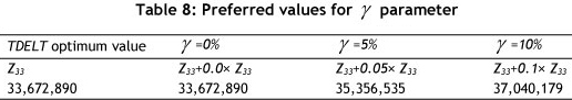
To solve problem 2, first the γ parameter must be calculated based on the DMs' preferences for the right-hand side of the new constraint (TDELT). Table 8 shows three preferred values for the delivery time performance index ( γ ).

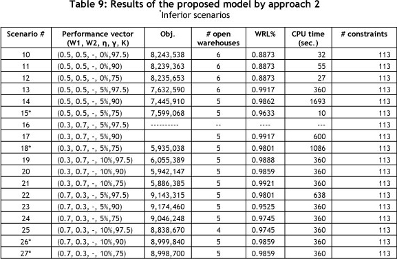
Based on three values for W₁, W₂ and γ, eighteen scenarios have been generated. The results of these scenarios are presented in Table 9. In approach 2, the WRL average (0.9644) is lower than approach 1 (0.9865); and by considering the TDELT objective in approach 2, this effect was predictable. Considering the sixth column in Table 8, it can be determined that since Z_p2 is a non-linear objective, the range of the CPU time to solve this problem is very wide, from 32 to 1,693 seconds. Comparing the CPU times in Table 6 and 9 shows that these times for problem 2 are significantly larger than those for problem 1. Unfortunately, LINGO optimisation software could not solve the 16^th scenario in 180 minutes. The results presented in Table 9 are illustrated graphically in Figures 4 and 5.

 

 

 

 

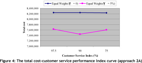
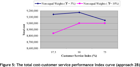
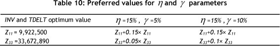
Table 10 shows the preferred values for η and γ in problem 3. For this problem, six scenarios are examined. The performance vectors and the other results are presented in Table 11, and illustrated graphically in Figure 6. It is interesting to note that in approach 3 the WRL average is 0.9878, and it is higher than the other approaches.

 

 

In summary, we make the following observations from our case analysis:

• Ten cases out of 33 scenarios are dominated by the other ones.
• The solution results indicate that the proposed model is not very sensitive to CSPI, so the preferred value for this parameter is 97.5%.

It can be concluded that the proposed SGP solution using approach 3 may provide different and even more preferable results when compared with approaches 1 and 2

 

6. SUMMARY AND CONCLUSION

This study proposed a multi-objective, multi-commodity distribution planning model that integrates location and inventory control decisions in a multi-echelon supply chain network with multiple capacity centres in a stochastic environment. An interactive stochastic goal programming formulation for food production is developed. The goal of the model is to select the optimum numbers, locations, and capacity levels of the warehouses to deliver the products to the retailers at the least cost, while satisfying the desired service level. The modelling approach of this model is distinguished from the other models in this field by the fact that DMs' imprecise aspiration levels for the goals, and retailers' imprecise demand are incorporated into the model using a stochastic modelling approach, which is otherwise not possible by conventional mathematical programming methods.

This paper also contributes to the literature by proposing a novel and generic SGP-based solution approach that determines the preferred compromise solution for multi-objective decision problems.

An Iranian food industry case study was used to demonstrate the feasibility of the proposed method for real distribution problems. Some realistic scenarios have been investigated, based on the DMs' strategies. These strategies can be compared by determining the performance vector for each strategy. The proposed method yields an efficient solution and overall degree of DMs' satisfaction with the determined objective values. Accordingly, the proposed method is practically applicable to solving real-world multi-objective DPD problems in an uncertain environment.

 

ACKNOWLEDGMENT

The authors would like to thank Prof. S.A. Torabi for his valuable and constructive suggestions on this work, which improved the content substantially.

 

REFERENCES

[1] Liang, T.F. 2006. Distribution planning decisions using interactive fuzzy multi-objective linear programming, Fuzzy Sets and Systems, 46, 1303-1316.         [ Links ]

[2] Torabi, S.A. & Hassini, E. 2008. An interactive possibilistic programming approach for multiple objective supply chain master planning, Fuzzy Sets and Systems, 159, 193-214.         [ Links ]

[3] Snyder, L.V. 2006. Facility location under uncertainty: A review, IIE Transactions, 38, 537-554.         [ Links ]

[4] Farahani, R.Z. & Elahipanah, M. 2008. A genetic algorithm to optimize the total cost and service level for just-in-time distribution in a supply chain, International Journal of Production Economics, 111, 229-243.         [ Links ]

[5] Miranda, P.A. & Garrido, R.A. 2004. Incorporating inventory control decisions into a strategic distribution network design model with stochastic demand, Transportation Research Part E, 40, 183-207.         [ Links ]

[6] Miranda, P.A. & Garrido, R.A. 2008. Valid inequalities for Lagrangian relaxation in an inventory location problem with stochastic capacity, Transportation Research Part E, 44, 47-65.         [ Links ]

[7] Daskin, M.S., Coullard, C.R. & Shen, Z-J.M. 2002. An inventory-location model: Formulation, solution algorithm and computational results, Anna's of Operations Research, 110, 83-106.         [ Links ]

[8] Shen, Z.-J.M., Coullard, C. & Daskin, M.S. 2003. A joint location-inventory model, Transportation Science, 37(1), 40-55.         [ Links ]

[9] Erlebacher, S.J. & Meller, R.D. 2000. The interaction of location and inventory in designing distribution systems, IIE Transactions, 32, 155-166.         [ Links ]

[10] Selim, H. & Ozkarahan, I. 2008. A supply chain distribution network design model: An interactive fuzzy goal programming-based solution approach, Internationa' Journa' of Advanced Manufacturing Technology, 36(3-4).         [ Links ]

[11] Gourdin, E., Labbe, M. & Laporte, G. 2000. The uncapacitated facility location problem with client matching, Operations Research, 48, 671-685.         [ Links ]

[12] Jayaraman, V. 1998. An efficient heuristic procedure for practical sized capacitated warehouse design and management, Decision Sciences, 29L, 729-745.         [ Links ]

[13] Pirkul, H. & Jayaraman, V. 1998. A multi-commodity, multi-plant, capacitated facility location problem: Formulation and efficient heuristic solution, Computers & Operations Research, 25(10), 869-878.         [ Links ]

[14] Tragantalerngsak, S., Holt, J. & Ronnqvist, M. 2000. An exact method for the two-echelon, single-source, capacitated facility location problem, European Journal of Operational Research, 123, 473-489.         [ Links ]

[15] Amiri, A. 2006. Designing a distribution network in a supply chain system: Formulation and efficient solution procedure, European Journal of Operational Research, 171, 567-576.         [ Links ]

[16] Hunt, I., Wall, B., & Jadgev, H. 2005. Applying the concepts of extended products and extended enterprises to support the activities of dynamic supply networks in the agri-food industry, Journal of Food Engineering, 70, 393-402.         [ Links ]

 

 

* Corresponding author

 

 

APPENDIX

In this appendix we proof Eq. 2:

A1. Stochastic weights in allocation problem: Transportation costs

In this section we used the Weber problem for modelling allocation/transportation costs. The objective allocation function is:

where wil is the weights of the demand customer zone i for product ' and d( Xj, Pi) is the distance between customer zone i , located at P' =(a¡ , b) and the warehouse j located at X= (Xj, y_j). We consider the following Euclidean distance measure:

Since w_il' is a stochastic parameter, the allocation costs function to be minimised is:

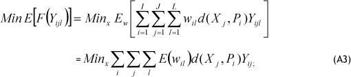
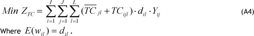
To calculate transportation costs, we replaced the distance component in the above objective function with the transportation cost in the whole network. Now we can formulate the transportation costs objective function, which is equivalent to:

A2. Inventory holding costs

To calculate inventory holding costs at any located warehouse, we consider the continuous inventory revision [5]. In this inventory control policy, when the inventory level of product l falls below r_jt , an order of Qj_t units is triggered, which is received after LT_jt time units. Figure A1 shows the stochastic demand pattern and warehouse fulfil rate. In this figure, the continuous line is the on-hand inventory, and the segmented line is the inventory position.

 

 

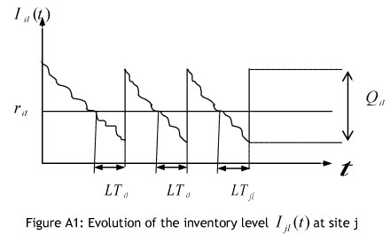
If an order is submitted to any located warehouse, the inventory level must cover the customers' demand during lead time LTjl , with a given probability 1 - α from the DMs.

This probability is known as the service level of the inventory system. The service level constraint can be written as follows:

where D(LT}1) is the uncertain demand, assigned to the warehouse j during the lead time for product l, and d_max(jl) is maximum demand during the lead time, and can be expressed as follow:

where is the mean demand, assigned to warehouse j during the lead for product ', and ssι is the level of safety stock inventory that should be held at warehouse j for product l.

If we assume a normal distribution demand, and consider d_max(jl) as the re-order point, j can be determined as follows:

Since in this paper we assume that the LTj' is a constant parameter, then Eq. (A7) is:

where Z_1-a is the value of the standard normal distribution, which accumulates a probability of 1 - α . This parameter is assumed to be fixed for the entire network, determining a uniform service level of the system.

The average holding cost rate for each warehouse j and product ' ($/day) based on Eq. (A8), can be written as:

The first term of Eq. (A9) is the average cost incurred due to holding the order quantity Q_jl, which is the inventory of product ' used to cover the demand that arose during two successive orders. The second term in (A9) is the average cost associated with safety stock kept at warehouse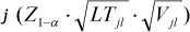

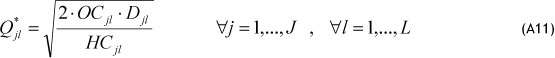
In this case we assume that there is no capacity constraint on the order quantity. So, differentiating the objective function in terms of Qj_t for each warehouse and product, and equaling to zero, we get:

From Eq. (A10) we could obtain:

By replacing Eq. (A11) in Eq. (A9), the TCOST objective function can be expressed as follows: