Quantitative and qualitative methods in risk-based reliability assessing under epistemic uncertainty

 

 

M. Khalaj^{I, *}; A. Makui^II; R. Tavakkoli-Moghaddam^III

^IDepartment of Industrial Engineering Science and Research Branch, University of Islamic Azad University, Tehran, Iran mehran5_k@hotmail.com
^IIDepartment of Industrial Engineering Iran University of Science and Technology, Tehran, Iran amakui@iust.ac.ir
^IIIDepartment of Industrial Engineering College of Engineering, University of Tehran, Tehran, Iran tavakoli@ut.ac.ir

 

 

---

ABSTRACT

The overall objective of the reliability allocation is to increase the profitability of the operation and optimise the total life cycle cost without losses from failure issues. The methodology, called risk-based reliability (RBR), is based on integrating a reliability approach and a risk assessment strategy to obtain an optimum cost and acceptable risk. This assessment integrates reliability with the smaller losses from failures issues, and so can be used as a tool for decision-making. The approach to maximising reliability should be replaced with the risk-based reliability assessment approach, in which reliability planning, based on risk analysis, minimises the probability of system failure and its consequences. This paper proposes a new methodology for risk-based reliability under epistemic uncertainty, using possibility theory and probability theory. This methodology is used for a case study in order to determine the reliability and risk of production systems when the available data are insufficient, and to help make decisions.

---

OPSOMMING

Die hoofdoelwit van betroubaarheidstoedeling is die verhoging van winsgewendheid van sisteemgebruik teen die agtergrond van optimum totale leeftydsikluskoste. Die metodologie genaamd "risikogebaseerde betroubaarheid" behels die bepaling van 'n risikoskatting om optimum koste te behaal vir 'n aanvaarbare risiko. Die navorsing stel vervolgens 'n nuwe ontledingsmetode voor vir epistemiese onsekerheid gebaseer op moontlikheids- en waarskynlikheidsleer. 'n Bypassende gevallestudie word aangebied.

---

 

 

Nomenclature

m             mass function

bpa          basic probability assignment

bel           belief function

pl             plausibility function

doubt       doubt function

C             total system cost

C_i(R_i)        cost of component/subsystem i

R_i             reliability of component/subsystem i

n              number of components within the system considered in the optimisation

R_1,min       minimum reliability of component/subsystem i

Ri,_max       maximum achievable reliability ofcomponent/subsystem i

R_s            system reliability

R_G            system reliability goal

 

1. INTRODUCTION

Avoiding the risks of a production system by increasing reliability is the main goal of this study. In recent years there has been an increased emphasis on accounting for the various forms of uncertainties that are introduced in mathematical models and simulation tools. Various forms of uncertainties exist, and it is very important that each one of them is accounted for, depending on the amount of available information.

Gathering data for reliability is mostly done under uncertain conditions that may be simplified. This type of uncertainty, known as epistemic uncertainty, occurs as a result of a lack of knowledge. Risk has two dimensions: 1) the severity of the consequences of the event, and 2) the probability of its occurrence. In the case of a production system, one can use a reliability index to calculate the likelihood of failure; but there is an even larger lack of knowledge regarding consequences.

In this paper, an integrated method is proposed to determine risk-based reliability in uncertain conditions. It attempts to determine epistemic uncertainty using intervals bounding variables. Some applications of intervals variables are available in the literature -for instance, as upper and lower coherent methods of prediction [11, 17].

In general, several methods are used to predict the future, notably possibility theory [5], evidence theory [4], the transferable belief model [14], and Bayesian theory [1]. However, the method used in this paper is the Dempster-Shafer theory [4], which is normally used for decision-making under uncertainty conditions and when rarely-found data related to our subject of decision are used. The application of this method helps to use the maximum data available and to calculate the maximum risk in predicting the reliability of systems under epistemic uncertainty conditions. This means that, instead of seeking a precise number, we determine the range. For instance, to determine the consequence of a system failure, we produce a range rather than a particular number. This study aims to calculate risk-based reliability under uncertainty conditions. It employs the Dempster-Shafer theory to describe the relation between reliability and system-failure risk, and finally to find the minimum and maximum required reliability for a production system, while coming to a certain decision using the minimum available data. The problem of risk and reliability estimations is an old problem; and the difficulty of reliability optimisation risk and reliability needs accurate modelling and accurate data. But accurate data are not always available; therefore, we can only strive towards a hybrid optimal reliability strategy that consists of qualitative and quantitative methods.

 

2. RISK-BASED RELIABILITY (RBR)

A considerable number of studies have introduced reliability optimisation involving costs [6, 10, 15, 18]. On the other hand, a risk-based method aims at reducing the overall risk that may result as a consequence of the unexpected failure of operating facilities. By assessing- the level of reliability of each component, one can prioritise the risk caused by the failure for the components of the system. It means that high risk items are given more reliability allocation than low risk items. Using risk-based reliability (RBR), one can determine the reliability allocation of equipment to minimise the total risk as a result of failure. The implementation of RBR reduces the likelihood of an unexpected failure through estimate and adjustment reliability.

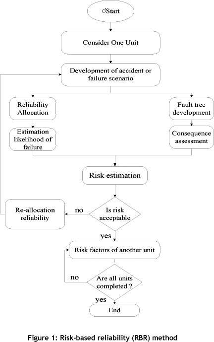
The minimum optimum reliability of the system can be found by creating a balance between the cost of a system failure and the cost of finding reliability [8]. The quantitative value of the risk is the basis for prioritising the improvement reliability activities, and is shown in Figure 1. RBR starts by separating the complete system under study into small manageable units. The risk, which is computed for a specific failure scenario(s) of a unit, is compared and evaluated against the acceptance criteria. If the risk value exceeds the criteria, the reliability allocation is re-evaluated for the optimal cost that brings the exceeded risk to an acceptable level. This process is repeated for each unit. The results obtained for all units are combined to develop a reliability allocation plan for the system. A description of each step of the RBR method is detailed in the following sections and case study.

 

 

3. DECISION-MAKING UNDER UNCERTAIN CONDITIONS

In recent decades, much attention has been given to various methods of making a decision under uncertain conditions. Among these methods, the belief theory, known as the Dempster-Shafer theory, is capable of showing and representing the uncertainty of our incomplete knowledge. The application of this theory was based on Dempster's work in explaining the principles of calculating upper and lower probabilities [4], and then the mathematical theory developed by Shafer [13]. In recent decades, the Bayesian statistical theory was used by many researchers in the literature because it was a well-known theory in this area. However, a few studies have been carried out in the Dempster-Shafer theory recently. Dempster-Shafer studies have a wide range of applications as a technique for modelling under uncertain conditions. Various studies are introduced for uncertainty management. Buchanan & Shortliffe [2] introduced a model that manages uncertainty and has certain factors. With limited knowledge, it is more suitable to use uncertain methods. Fedrizzi & Kacprzyk [7] carried out a number of studies on fuzzy prioritising and on using the interval value to show the opinions and judgment of experts through accumulated distributions. Every method that we use for uncertainty management has its own advantages and disadvantages [12]. For instance, Walley [l6] and Caselton & Luo [3] discussed problems resulting from the Bayes's popular analysis, caused by the lack of information. Klir [9] carried out a critical analysis of uncertainty for gaining knowledge.

Among the above-mentioned methods, the Dempster-Shafer theory [4] has been widely used when the data have been gathered from several sources. In this study the Dempster-Shafer theory is also used to calculate the failure risk of equipment in a production organisation. What happens to production systems in a real situation is not predictable. One is always confronted with risk, especially when the data is limited. Although various studies have been carried out into using Dempster-Shafer theory in identifying systems, calculating, and decision-making, one is still confronted with problems in the practical use of the theory in assessing the existing risk of the system and in making executive decisions in real production systems. The study aims to propose an integrated method for the better identification of risk assessment of equipment, and making it practicable. The executive samples are also provided by calculating the risk of the facilities in a production organisation.

Yager [19] stated that if one cannot obtain the exact probability, one can estimate the rank of the probability, as shown below.

The above equation is the core of this study. With it, the risk and reliability of a production system under uncertain conditions may be calculated.

3.1 Basic probability assignment

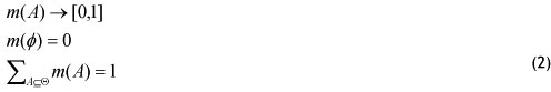
The basic probability assignment (BPA or m) differs from the classical definition of probability. It is defined by mapping over the interval [0-1], in which the basic assignment of the null set m(o) is zero, and the summation of basic assignments in a given set A is '1'. The basic probability assignment is called a focal element for each element for which m (A) * 0 is true. This can be represented by:

3.2 Belief function

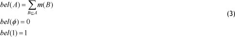
The lower and upper bounds of an interval can be determined through a basic probability assignment, which includes the probability of the set bounded by two non-additive measures, namely belief and plausibility. The lower limit of belief for a given set A is defined as the summation of all basic probability assignments of the proper subsets B, in which B is a subset of A. The general relation between BPA and belief can be represented by:

3.3 Plausibility function

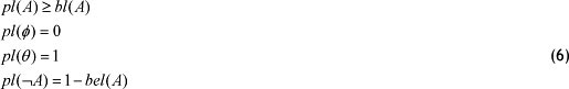
The upper bound is plausibility, which is the summation of basic probability assignments of subsets of B, for which A (i.e., BHA * 0) is true, and is expressed by:

The plausibility function is related to the belief function through the doubt function, defined by:

Moreover, the following relationship is true for the belief function and the plausibility function under all circumstances.

3.4 Belief interval

The belief interval represents a range in which the probability may lie. It is determined by reducing the interval between plausibility and belief. The narrow uncertainty band represents more precise probabilities. The probability is uniquely determined if bel(A)=pl(A); and for the classical probability theory, all probabilities are unique. If U(A) has an interval [0, 1], it means that no information is available; but if the interval is [1, 1],then it means that A has been completely confirmed by m(A).

 

4. RELIABILITY OPTIMISATION MODEL

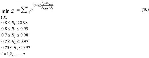
To compute the probability that all involved components are operational during the task several methods of allocation problem are available. This paper addresses the nonlinear optimisation problem by Tilman et al. [15] as follows:

It is clear from the above discussion that maximising the reliability of a distributed system is equivalent to minimising the unreliability cost function Z. However, to achieve a satisfactory allocation, additional constraints should be considered with the cost function to meet the application requirements and not to violate the availability of system resources.

Tilman et al. [15] obtain a relationship for the cost of each component as a function of its reliability. A general behaviour for the cost function is proposed as follows:

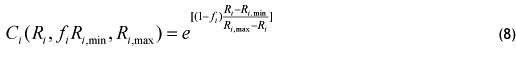
This formulation is applied to achieve three goals that are proved in the real conditions of a production system, as follows:

1. If a high reliability component is required, the related cost will be increased exponentially.

2. If a high reliability component is not required, the cost of a low reliability component will be low.

3. Increasing component reliability may be feasible or non-feasible.

In Eqs.(7) and (8), R^_min is the initial (current) reliability value of the ith component obtained from the failure distribution of that component and for the specified time. R_i,max, is the maximum achievable reliability of the ith component, and f_i is the feasibility of increasing a component's reliability, and it assumes values between 0 and 1.

To gain a level of reliability, one needs to know its feasibility. These features, depending on the complexity of the system, are gained through various methods such as a new reliability allocation through investments in process facilities. The greater the reliability of the systems, the greater the effort required; therefore, reliability improvement can be very difficult, costly, or impossible, depending on whether the design complexity, technological limitations, and feasibility parameter are a constant. It is difficult to improve the reliability of the component subsystem, since it is a number between 0 and 1.

This is an optional step, aimed at verifying that the reliability plan developed will produce an acceptable risk level for the complete system. In this step, the process is repeated using revised values for the failure probabilities. The result of this step determines whether or not the developed reliability plan is effective in managing risk.

 

5. CASE STUDY: OPTIMUM RBR STRATEGY FOR A PRODUCTION SYSTEM

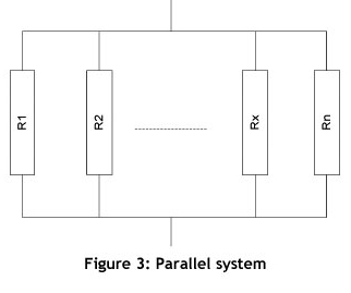
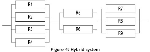
For the purposes of this study, any production system may be assigned to one of the following three categories: series systems (Figure 2), parallel systems (Figure 3), or hybrid systems (Figure 4).

 

 

 

 

 

 

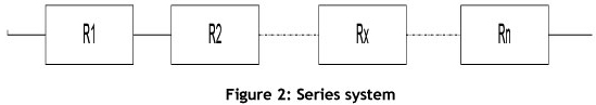
Series systems are those systems in which the failure of any element leads to the failure of the system. Conceptually, a series system is one that is as weak as its weakest link. A graphical description of a series system is shown in Figure 2.

A parallel system is a configuration in which, as long as not all of the system components fail, the entire system works. Conceptually, in a parallel configuration the total system reliability is higher than the reliability of any single system component. A graphical description of a parallel system of 'n' components is shown in Figure 3.

If a system does not satisfy these strict definitions of series or parallel systems, the system is classified as a hybrid system. Hybrid systems are made up of combinations of several series and parallel configurations. The way to obtain system reliability in such cases is to break the total system configuration down into homogeneous subsystems, and then to consider each of these subsystems separately as a unit, and calculate their reliabilities. Finally, put these simple units back (via series or parallel recombination) into a single system and obtain its reliability. A graphical description of a hybrid system is shown in Figure 4.

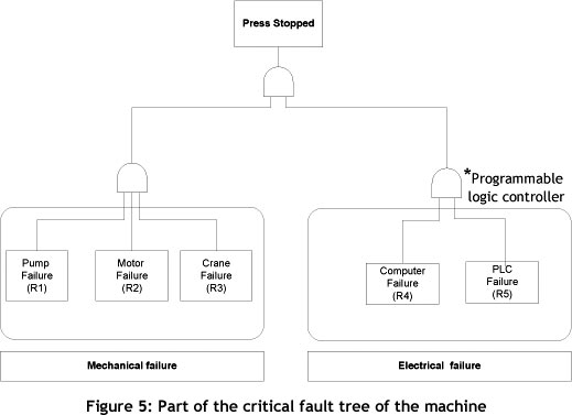
For example, consider a system composed of a combination in series. Assume that the objective reliability for the system is shown in Table 1 for a mission time of 150 hrs. To begin the analysis, part of the critical fault tree of the machine has been drawn (Figure 5). The first step is to obtain the system's reliability equation. In this case, and assuming independence, the reliability of the system, Rs, is given by:

 

 

 

 

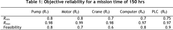
To represent the behaviour of the reliability function for each individual component using the cost function given by Eq. (8), a scenario is considered for the allocation problem of Table 1. There are three parameters in Table 1. R¡,_m¡„ is the minimum reliability of component/subsystem I, R_i,_max is the maximum achievable reliability of component/ subsystem i, and Feasibility is the feasibility of increasing the reliability of component/ subsystem i.

According to Table 1, by using Eq.7 it follows that:

The results for this case are shown in Table 2. It can be seen that the highest reliability is allocated to the component with the higher cost. When estimating the probability of the occurrence of an event (Probability of Failure, or POF), Reliability is always one at the start of its life (i.e., R(0) =1 and R(~) =0). If T is the time to failure, let R(t) be the probability P(T < t) that the time to failure T will not be greater than a specified time t. The time to failure distribution R (t) is linked with the probability of failure (POF) by:

 

 

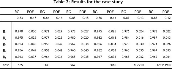
Subsequently one calculates reliability and POF as shown in Table 2 by using Eq. (10).

5.1 Application of the Dempster-Shafer calculations for consequence assessment

The objective here is to quantify the potential consequences of total functional failure, represented by a credible scenario. Although some data pertaining to the failure probability of systems is available, there is not adequate data for calculating the failure probability through the classical probability theory, since there are conditions of uncertainty. The analysis applies the Dempster-Shafer theory, resulting in a decision-making framework using the minimum available data, which includes an assessment of the likely consequences if a failure scenario did materialise.

With this method, the consequences are quantified in terms of damage by using a basic probability assignment instead of classical probability theory. Since one cannot use classical probability theory, use is made of intervals for determining the breakdown of machines. This allows one to distinguish the prioritisation performed on each category.

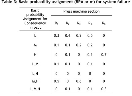
5.2 Basic probability assignment for consequence impact

The second factor in determining the risk of equipment is to find the magnitude of breakdowns. Existing data on failures during the previous 13 years are limited, and direct decision-making is not possible through statistical methods.

The company intends to make decisions about how to react to the failure risk of these three parts on the basis of previous data and expert opinion. After analysing the past records of breakdowns, they are sorted into three categories: (L) or low, in which the magnitude of breakdown is low; (M) or medium, where the magnitude of breakdown is medium and leads to interruption, but is repairable; and (H) or High, in which the magnitude of breakdown is high and, if it happens, will cause a crisis.

The set of occurrences will be Θ= {L, M, H}. There will be eight possible subsets: {φ},{L},{M},{H},{L,M},{L,H},{M,H},{L,M,H}. The set of basic probability allocations for the occurrence of breakdown in the production system is shown in Table 3. The gathered data on the magnitude of breakdown of machines are found in BPA's records of machine breakdown.

 

 

5.3 Calculation of failure consequence

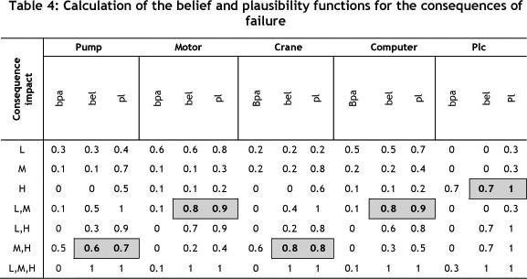
The upper and lower bounds of an interval are set by basic probability allocations, which include a probability set bounded by the two extents of belief and plausibility. The lower bound of belief (bel) from a given set A is the summation of all basic probabilities that are allocated to occurrences in Eq. (3), and the upper bound is also found through Eq. (4).

The probability interval found through the belief and plausibility functions represents an uncertain interval, which can be given by the correct value to wrong value due to lack of adequate data. The uncertain interval is between these two values. This interval starts from the belief function and continues to the value of the plausibility function. By using this interval U(A), the narrower U(A) shows an exact probability. In the analysis of the attained results of the belief and plausibility functions, if belief is equal to plausibility, the exact value for probability of failure consequence is obtained and then the uncertainty will be zero. In addition by using Eqs. (3) and (4), one can simply find the belief and plausibility functions for the system failure. Table 4 shows the results.

 

 

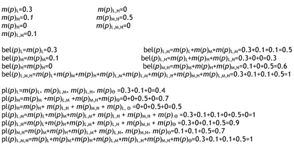
To determine the failure consequence of each machine from the table of belief and plausibility functions, the interval that has a large belief interval will be chosen, since the belief function determines a low probability that is gained through the minimum available data. For example, one can calculate the basic probability assignment (BPA or m) for the likelihood of failure consequence as follows:

The BPA for the pump or 'p' obtained from Table 4 is as follows:

 

 

After obtaining Tables 4 for all devices, a decision may be made by using the principles of Dempster-Shafer. The belief function bel(A) measures the total probability that must be distributed among the elements of A; it inevitability reflects and signifies the total degree of belief of A, and constitutes a lower limit function on the probability of A. On the other hand, the plausibility function pl(A) measures the maximal amount of probability that can be distributed among the elements in A; it describes the total belief degree related to A, and constitutes an upper limit function on the probability of a belief interval [bel(A), pl(A)]. Marked gray in Table 4, it reflects uncertainty and describes the unknown with respect to A. As shown in Table 4, different belief intervals represent different meanings.

A decision is made for the interval that must follow rules, such as the less uncertainty interval between belief and plausibility representing greater precision. Obtaining a belief function that considers the available evidence, the selected range has a higher belief.

5.4 Determining risk interval using risk assessment matrix

Once the failure probability and the magnitude band of system failure are determined, one can use the risk assessment matrix to find the level of risk for each component. For this purpose, a model may be used that assigns probability of failure and consequence impact in a band (Table 5).

 

 

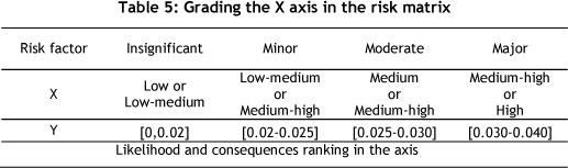
The grading of the band starts from insignificant breakdowns and ends with major breakdowns. After blending the two dimensions of Table 5, and drawing a two-dimensional risk diagram, it is found that the X axis of the diagram is related to the consequences, while the Y-axis shows the likelihood of the occurrence of failure or probability of failure (POF), in which each section represents the failure risk of each machine. For instance, calculations for a pump (R1), motor (R2), and PLC (R5) are shown in Figure 6.

 

 

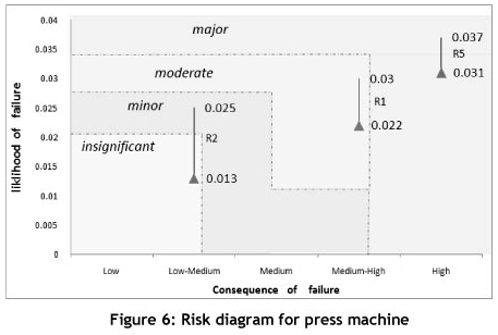
This figure indicates that the failure risk of the motor (R2) for two reliability intervals [R2=0.975 (i.e., F=0.025), R2=0.987 (i.e., F=0.013)] changes from minor risk to insignificant risk. Other results pertaining to other machines (i.e., pump and PLC) are shown in the diagram as well. The reliability of R1 for pump up to 0.978 can be increased. Thus, the probability of failure up to 0.022 can be decreased. Next, the risk of the pump is decreased; however, for the PLC, increasing the reliability does not affect on the risk. Thus, we should reduce the consequence impact of failure. For example, one can decrease the consequence impact with added redundancy. If one does not have adequate data available, qualitative and precise numbers may be used together to calculate the risk. In this case study, due to lack of information, a range for the consequence impact is determined, and the probability of failure with the relation between risk and reliability is calculated.

 

6. CONCLUSIONS

The final challenge of reliability optimisation problems is to find a solution that improves reliability with lower cost and risk. However, maximising system reliability does not necessarily guarantee decreasing losses from failure. This does not comply with the general understanding and knowledge of the concept of reliability. Decision-making is a process in which a decision-maker predicts and evaluates the outcome using existing data, and chooses a certain solution to attain the objective. For complex systems, no theoretical model is available for analysing risk. This article proposes a framework for showing and representing the uncertainty of incomplete knowledge when calculating the risk of a production system. A new approach is proposed named 'risk-based reliability'. This approach is useful for decision-making; under conditions of uncertainty, decision-makers still have to decide what the best solution will be for their purposes.

Usually the algorithms of optimal reliability search are used to maximise reliability or minimise cost. However, there is one important problem in any process that decision-makers must analyse to identify the risk of solution. In this paper, the Dempster-Shafer theory has been applied to guide the selection of preferences to achieve the best solution, via risk-matrix diagrams that visualise and analyse the risk for any component. When the risk factor is high, one may replace system reliability with feasible reliability at minimum cost and risk of production.

The contributions of this paper are in the four main sections on reliability allocation. These are to calculate the likelihood of failure, the consequence of failure and the risk to the production system, and to reallocate reliability decreasing risk to an acceptable level.

The results are from a case study of a single sample production system. In this way, decision-makers can focus on risk and reliability together.

The original contributions of the work include risk-based reliability that in complex systems helps the decision-maker to choose a certain solution for attaining the objective. The Dempster-Shafer theory is used to obtain the required data, and then analyse the data and prepare a scenario of choices for the decision-maker. The decision-maker then makes a choice, and the decision-making process is complete.

 

REFERENCES

[1] Berger, J.O. 1985. Statistical decision theory and Bayesian analysis. New York: Springer, 109130.         [ Links ]

[2] Buchanan, B.J. & Shortliffe, E.H. 1975. A model of inexact reasoning in medicine, Mathematical Biosciences, 23: 351-379.         [ Links ]

[3] Caselton, W.F. & Luo, W. 1992. Decision making with imprecise probabilities, Dempster-Shafer theory and applications, Water Resources Research, 28 (12): 3071-3083.         [ Links ]

[4] Dempster A.P. 1967. Upper and lower probabilities induced by a multi-valued mapping. Annals of Mathematical Statistics, 38: 325-39.         [ Links ]

[5] Dubois, D. & Prade, H. 1998. Possibility theory is not fully compositional! A comment on a short note by H.J. Greenberg. Fuzzy Sets and Systems, 131-134.         [ Links ]

[6] Elegbede, A.O.C, Chu, C., Adjallah, K.H. & Yalaoui, F. 2003. Reliability allocation through cost minimization, IEEE Transactions on Reliability, 52(1): 106-111.         [ Links ]

[7] Fedrizzi, M. & Kacprzyk, J. 1980. On measuring consensus in the setting of fuzzy preference relations making with fuzzy sets. IEEE Transactions on Systems, Man, and Cybernetics, 10: 716723.         [ Links ]

[8] Hecht, H. 2004. Systems reliability and failure prevention, Artech House.         [ Links ]

[9] Klir, G.J. 1989. Is there more to uncertainty than some probability theorists might have us believe?, International Journal of General Systems, 15: 347-78.         [ Links ]

[10] Kuo, W. & Prasad, R. 2000. An annotated overview of system-reliability optimization, IEEE Transactions on Reliability, 49(2): 176-187.         [ Links ]

[11] Kyburg, H.E. 1998. Interval-valued probabilities. The Imprecise Probabilities Project.         [ Links ]

[12] Lee, N.S., Grize, Y.L & Dehnald, K. 1987. Quantitative models for reasoning under uncertainty in knowledge-based expert systems, Int. J. Intell Syst. 2:15-38.         [ Links ]

[13] Shafer, G. 1976. A mathematical theory of evidence. Princeton: Princeton University Press.         [ Links ]

[14] Smets, P. 2000. Belief functions and the transferable belief model. The Imprecise Probabilities Project.         [ Links ]

[15] Tillman, F.A., Hwang, C.L. & Kuo, W. 1985. Optimization of systems reliability, Marcel Dekker.         [ Links ]

[16] Walley, P. 1987. Belief-function representations of statistical evidence. Ann Stat 10, 741-761.         [ Links ]

[17] Walley, P. 1991. Statistical reasoning with imprecise probabilities. New York: Chapman & Hall.         [ Links ]

[18] Wattanapongsakorn, N. & Levitan, S.P. 2004. Reliability optimization models for embedded systems with multiple applications, IEEE Transactions on Reliability, 53(3): 406-416.         [ Links ]

[19] Yager, R. 1987. On the Dempster-Shafer framework and new combination rules, Information Sciences 41 (2): 93-137.         [ Links ]

 

 

* Corresponding author